Disturbance of Immune-Related Pathways between Normal and Tumor Tissues in Pan-cancer

The data were obtained from
https://pmc.ncbi.nlm.nih.gov/articles/PMC9856581/#app1-cancers-15-00342.
For demonstration purposes, we randomly selected five pathways.
The dataset can be downloaded from Data Repository.

data <- readxl::read_xlsx("real-world-data/datasource/pan-cancer-immune-pathways/pan-cancer-immune-pathways.xlsx", skip = 1L)
#> New names:
#> • `` -> `...3`
#> • `` -> `...5`
#> • `` -> `...7`
#> • `` -> `...9`
#> • `` -> `...11`
#> • `` -> `...13`
#> • `` -> `...15`
#> • `` -> `...17`
#> • `` -> `...19`
#> • `` -> `...21`
#> • `` -> `...23`
#> • `` -> `...25`
#> • `` -> `...27`
#> • `` -> `...29`
#> • `` -> `...31`
#> • `` -> `...33`
#> • `` -> `...35`
#> • `` -> `...37`
#> • `` -> `...39`
#> • `` -> `...41`
#> • `` -> `...43`
#> • `` -> `...45`
#> • `` -> `...47`
#> • `` -> `...49`
#> • `` -> `...51`

set.seed(3L)
# Randomly select 5 pathways (rows 2–18 cover the main data)
selected <- sample(2:18, 5)
# Extract logFC and adjusted p-values for the selected pathways
logFC <- data[selected, c(1, which(as.character(data[1, ]) == "logFC"))]
adj.P <- data[selected, c(1, which(as.character(data[1, ]) == "adj.P"))]
names(adj.P) <- names(logFC)

# Convert to numeric matrix: pathways as columns, tumor as rows
logFC <- dplyr::mutate(logFC, dplyr::across(!pathway, as.numeric)) |>
    tibble::column_to_rownames(var = "pathway") |>
    as.matrix() |>
    t()
adj.P <- dplyr::mutate(adj.P, dplyr::across(!pathway, as.numeric)) |>
    tibble::column_to_rownames(var = "pathway") |>
    as.matrix() |>
    t()

library(ggalign)
#> Loading required package: ggplot2
#> ========================================
#> ggalign version 1.2.0.9000
#> 
#> If you use it in published research, please cite: 
#> Peng, Y.; Jiang, S.; Song, Y.; et al. ggalign: Bridging the Grammar of Graphics and Biological Multilayered Complexity. Advanced Science. 2025. doi:10.1002/advs.202507799
#> ========================================

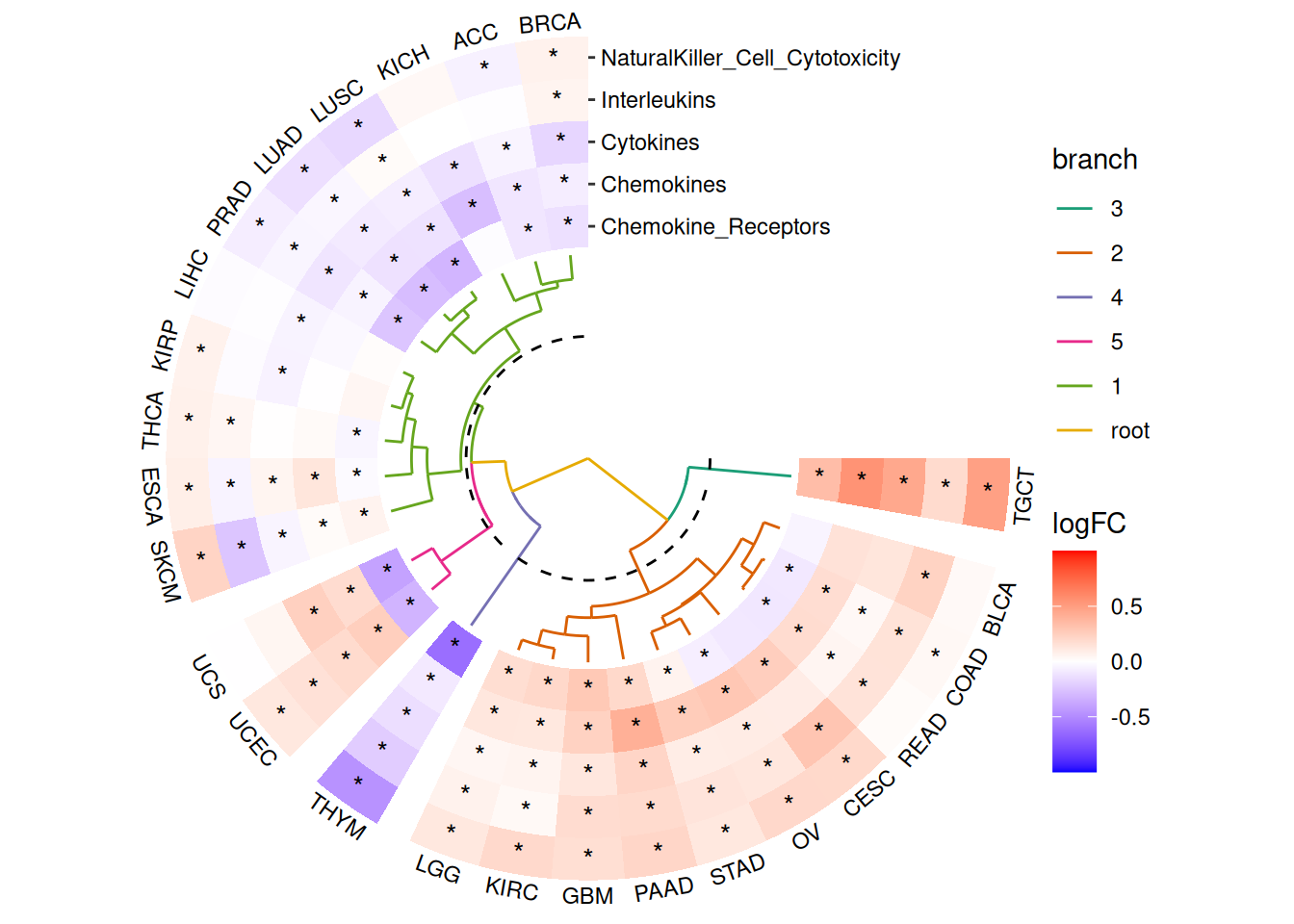
circle_discrete(logFC,
    radial = coord_radial(start = pi / 2, end = pi * 2, expand = FALSE),
    sector_spacing = 5 * pi / 180,
    theme = theme(plot.margin = margin(l = 5, t = 5, b = 6, unit = "mm"))
) +
    # Align dendrogram above the radial sectors, cluster conditions into 5 groups
    align_dendro(aes(color = branch), k = 5L, size = 1) +
    theme_no_axes("y") +
    scale_color_brewer(palette = "Dark2") +

    # add heatmap plot
    ggalign(mapping = aes(y = .column_names, fill = value)) +
    geom_tile(width = 1, height = 1) +
    geom_text(aes(label = "*"), data = function(dd) {
        dd$pvalue <- adj.P[cbind(dd$.row_index, dd$.column_index)]
        dplyr::filter(dd, pvalue < 0.05)
    }) +
    scale_fill_gradient2(
        low = "blue", high = "red",
        name = "logFC",
        limits = c(-1, 1),
        breaks = c(-0.5, 0, 0.5)
    ) +
    guides(r = "none", r.sec = "axis", theta = guide_axis_theta(angle = 0)) +
    theme(axis.text.theta = element_text())