11  Quad-side Layout

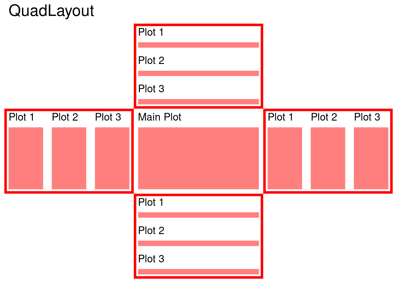
quad_layout() arranges plots around the quad-sides of a main plot, aligning both horizontal and vertical axes, and can handle either discrete or continuous variables.

library(ggalign)
set.seed(123)
small_mat <- matrix(rnorm(56), nrow = 7)
rownames(small_mat) <- paste0("row", seq_len(nrow(small_mat)))
colnames(small_mat) <- paste0("column", seq_len(ncol(small_mat)))

11.1 Introduction

Depending on whether you want to align discrete or continuous variables in the horizontal and vertical direction, there are four main types of quad_layout():

Alignment of Observations	horizontal	vertical	Data Format
quad_continuous()/ggside()	continuous	continuous	data frame
quad_layout(xlim = ...)	discrete	continuous	matrix
quad_layout(ylim = ...)	continuous	discrete	matrix
quad_discrete()/ggheatmap()	discrete	discrete	matrix

11.2 Annotations

Annotation is typically handled using a stack_layout(). Depending on whether you want to align observations in the specified direction, different stack_layout() are compatible (Section 7.5). Below is a table outlining the compatibility of various layout types for annotations:

Annotations	left and right	top and bottom
quad_continuous()/ggside()	stack_continuous()	stack_continuous()
quad_layout(xlim = ...)	stack_discrete()	stack_continuous()
quad_layout(ylim = ...)	stack_continuous()	stack_discrete()
quad_discrete()/ggheatmap()	stack_discrete()	stack_discrete()

11.3 quad_discrete()

quad_discrete() aligns discrete variables in both horizontal and vertical directions. It serves as the base version of ggheatmap()/heatmap_layout() and does not automatically add default layers or mappings.

The underlying ggplot data of the main plot is the same with ggheatmap()/heatmap_layout() (Section 7.2), it is recommended to use .y/.discrete_yas theymapping and use.x/.discrete_xas thex` mapping in the main plot.

quad_discrete(small_mat, aes(.x, .y)) +
    geom_tile(aes(fill = value)) +
    scale_fill_viridis_c()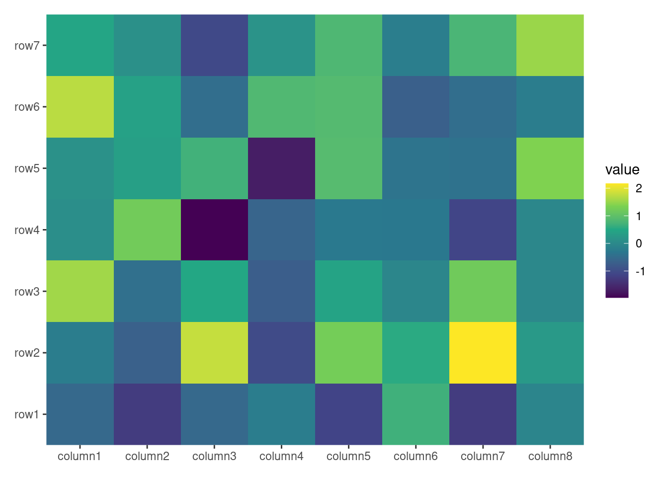

11.4 quad_continuous()

quad_continuous() align continuous variables and is functionally equivalent to the ggside package. For convenience, ggside() is provided as an alias for quad_continuous(). This layout is particularly useful for adding metadata or summary graphics along a continuous axis.

ggside(mpg, aes(displ, hwy, colour = class)) +
    geom_point(size = 2) +
    # initialize top annotation
    anno_top(size = 0.3) +
    # add a plot in the top annotation
    ggalign() +
    geom_density(aes(displ, y = after_stat(density), colour = class), position = "stack") +
    # initialize right annotation
    anno_right(size = 0.3) +
    # add a plot in the right annotation
    ggalign() +
    geom_density(aes(x = after_stat(density), hwy, colour = class),
        position = "stack"
    ) +
    quad_scope(theme_bw(), "tri")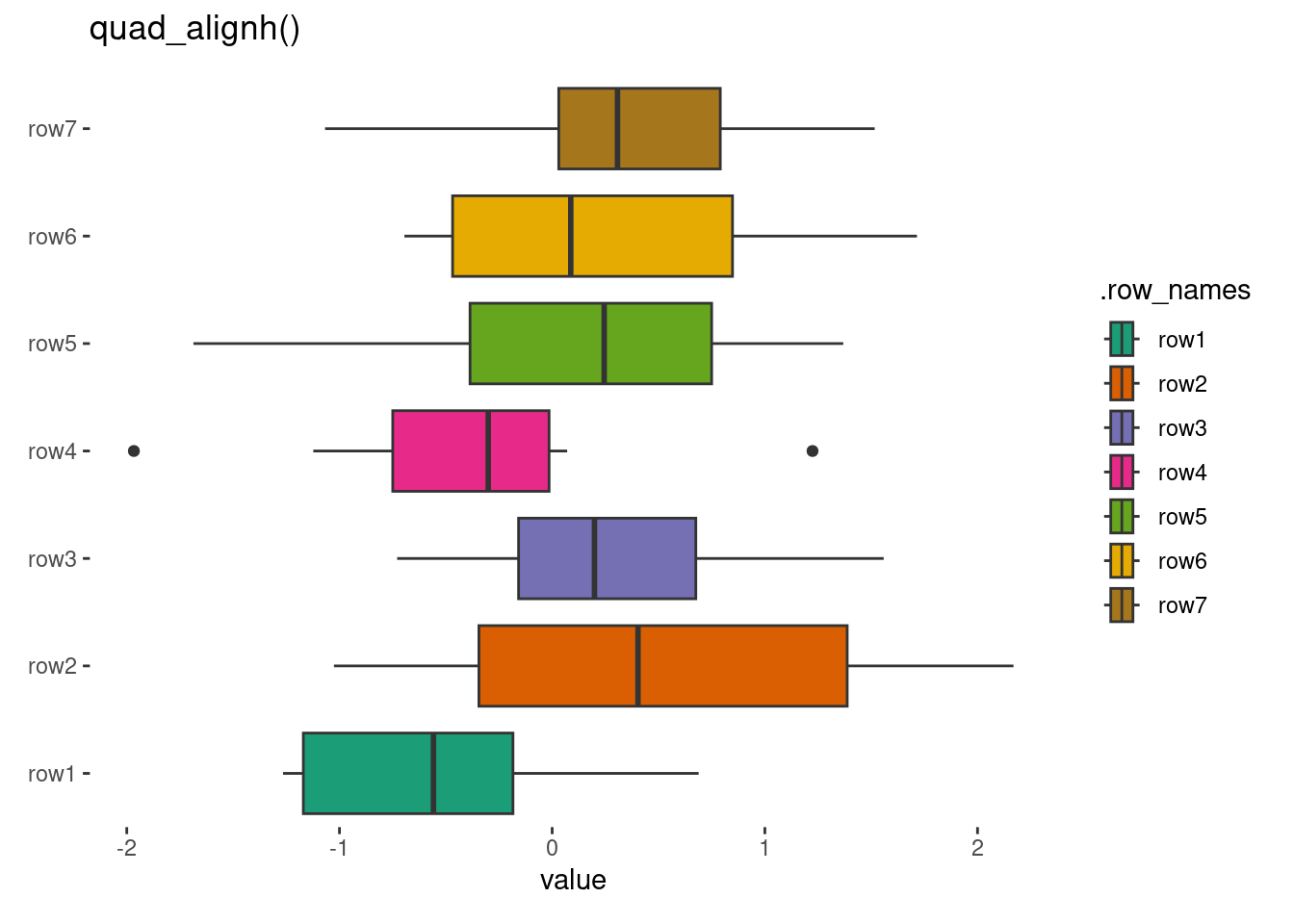

The quad_scope() function controls the active adding context. The "tri" argument means adding to the top annotation, right annotation, and the main plot. More details will be introduced in the Chapter 13 chapter.

ggside() allows facetting for the main plot, which should also be applied to the annotations for proper alignment.

i2 <- iris
i2$Species2 <- rep(c("A", "B"), 75)
ggside(i2, aes(Sepal.Width, Sepal.Length, color = Species)) +
    geom_point(size = 2) +
    facet_grid(Species ~ Species2) +
    anno_top(size = 0.3) +
    ggalign() +
    geom_density(aes(Sepal.Width, y = after_stat(density), colour = Species),
        position = "stack"
    ) +
    facet_grid(cols = vars(Species2)) +
    anno_right(size = 0.3) +
    ggalign() +
    geom_density(aes(x = after_stat(density), Sepal.Length, colour = Species),
        position = "stack"
    ) +
    facet_grid(rows = vars(Species)) +
    quad_scope(theme_bw(), "tri")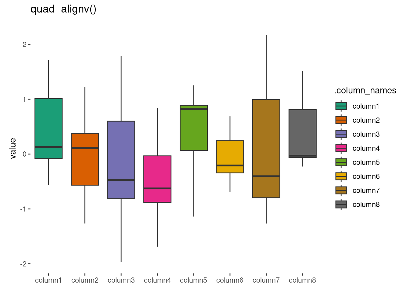

11.5 quad_layout()

This function arranges plots around the quad-sides of a main plot, aligning both horizontal and vertical axes, and can handle either discrete or continuous variables.

• If xlim is provided, a continuous variable will be required and aligned in the vertical direction. Otherwise, a discrete variable will be required and aligned.
• If ylim is provided, a continuous variable will be required and aligned in the horizontal direction. Otherwise, a discrete variable will be required and aligned.

quad_layout(small_mat, xlim = NULL) +
    geom_boxplot(aes(value, .discrete_y, fill = .row_names)) +
    scale_fill_brewer(palette = "Dark2") +
    layout_title("quad_layout(xlim = ...)")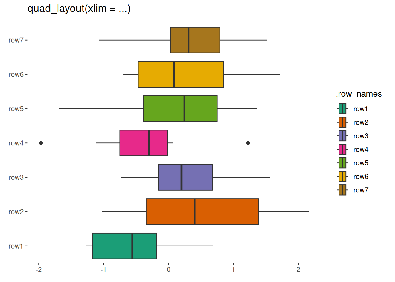

quad_layout(small_mat, ylim = NULL) +
    geom_boxplot(aes(.discrete_x, value, fill = .column_names)) +
    scale_fill_brewer(palette = "Dark2") +
    layout_title("quad_layout(ylim = ...)")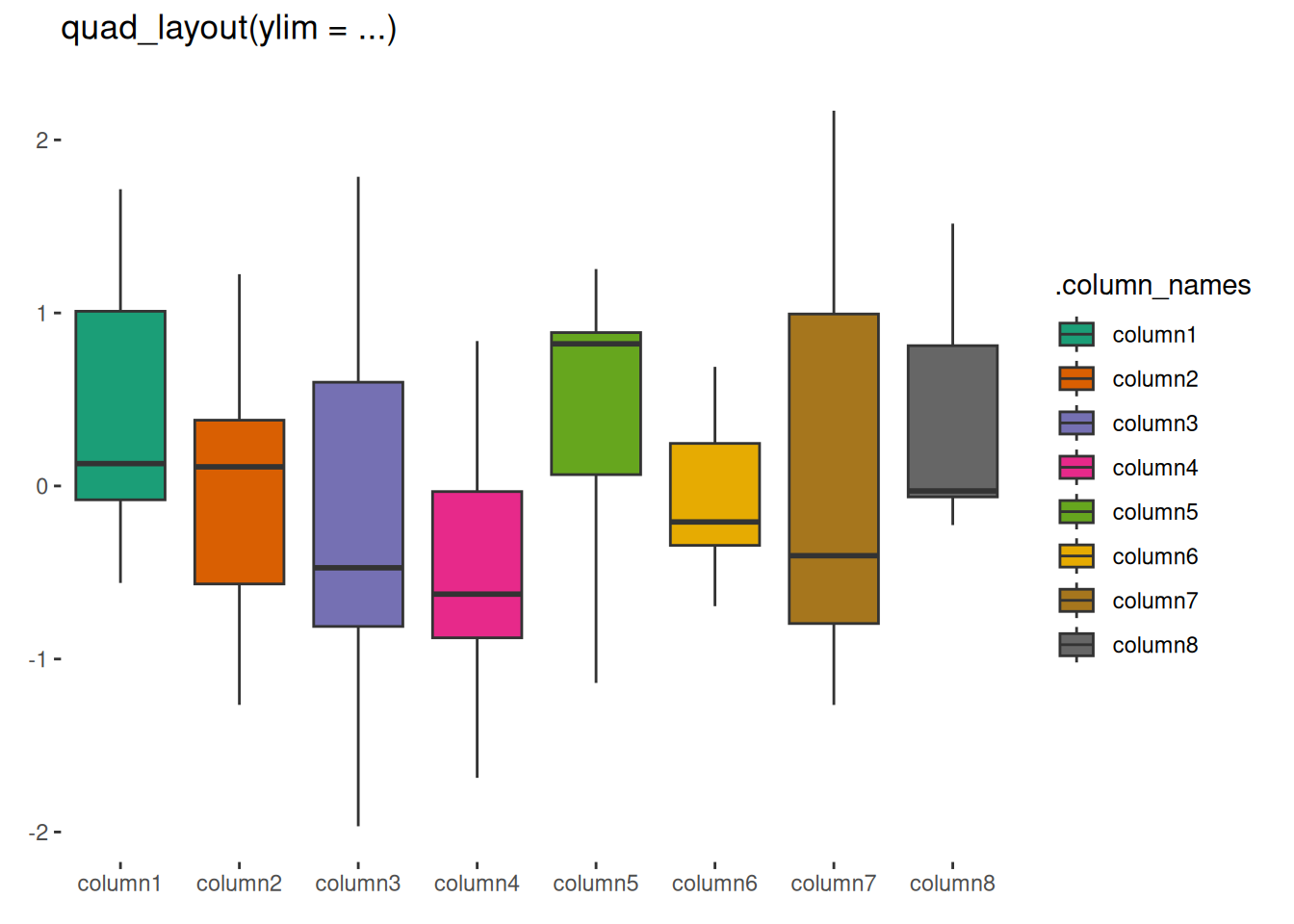

As discussed in Section 7.4, quad_anno() will always attempt to initialize a stack_layout() with the same alignment as the current direction. For top and bottom annotations in quad_layout(xlim = ...), and left and right annotations in quad_layout(ylim = NULL), quad_anno() will not initialize the annotation due to inconsistent data types.

quadh <- quad_layout(small_mat, xlim = NULL) +
    anno_top()
#> Warning: `data` in `quad_layout()` is a double matrix, but the top annotation stack need
#> a <data.frame>, won't initialize the top annotation stack
quadv <- quad_layout(small_mat, ylim = NULL) +
    anno_left()
#> Warning: `data` in `quad_layout()` is a double matrix, but the left annotation stack
#> need a <data.frame>, won't initialize the left annotation stack

Manual adding of a stack_layout() is required in such cases, you can set initialize = FALSE to prevent the warning message.

quadh <- quad_layout(small_mat, xlim = NULL) +
    anno_top(initialize = FALSE)
quadv <- quad_layout(small_mat, ylim = NULL) +
    anno_left(initialize = FALSE)

quadh +
    stack_continuous("v", mpg) +
    # add a plot in the top annotation
    ggalign(mapping = aes(displ, hwy, colour = class)) +
    geom_point(aes(displ, hwy, colour = class)) +
    quad_active() +
    geom_boxplot(aes(value, .discrete_y, fill = .row_names)) +
    scale_fill_brewer(palette = "Dark2")+
    layout_title("quad_alignh()")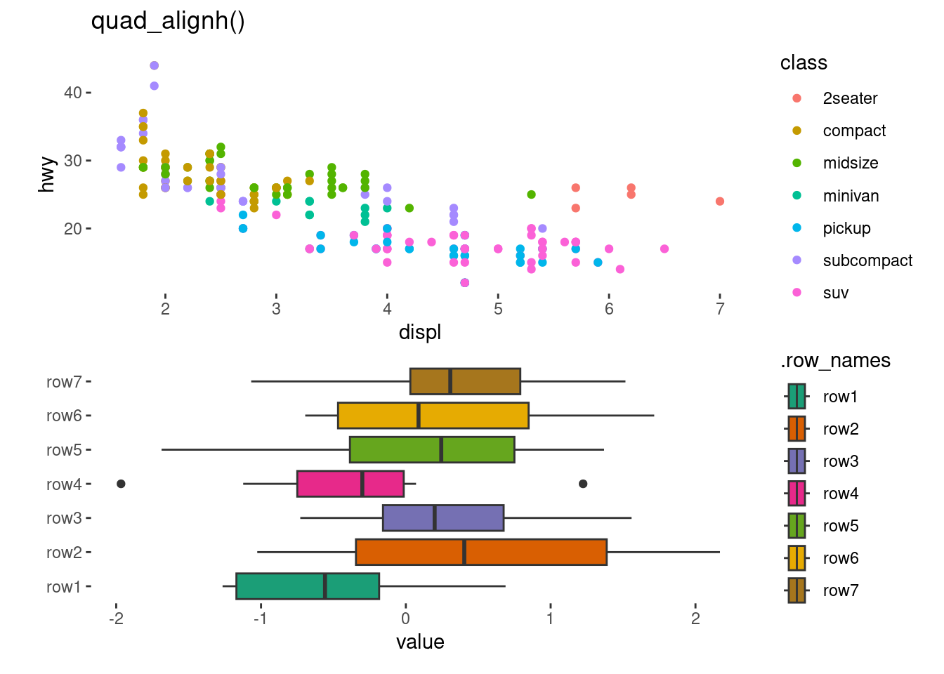

quadv +
    stack_continuous("h", mpg) +
    # add a plot in the left annotation
    ggalign(mapping = aes(displ, hwy, colour = class)) +
    geom_point(aes(displ, hwy, colour = class)) +
    quad_active() +
    geom_boxplot(aes(.discrete_x, value, fill = .column_names)) +
    scale_fill_brewer(palette = "Dark2") +
    layout_title("quad_alignv()")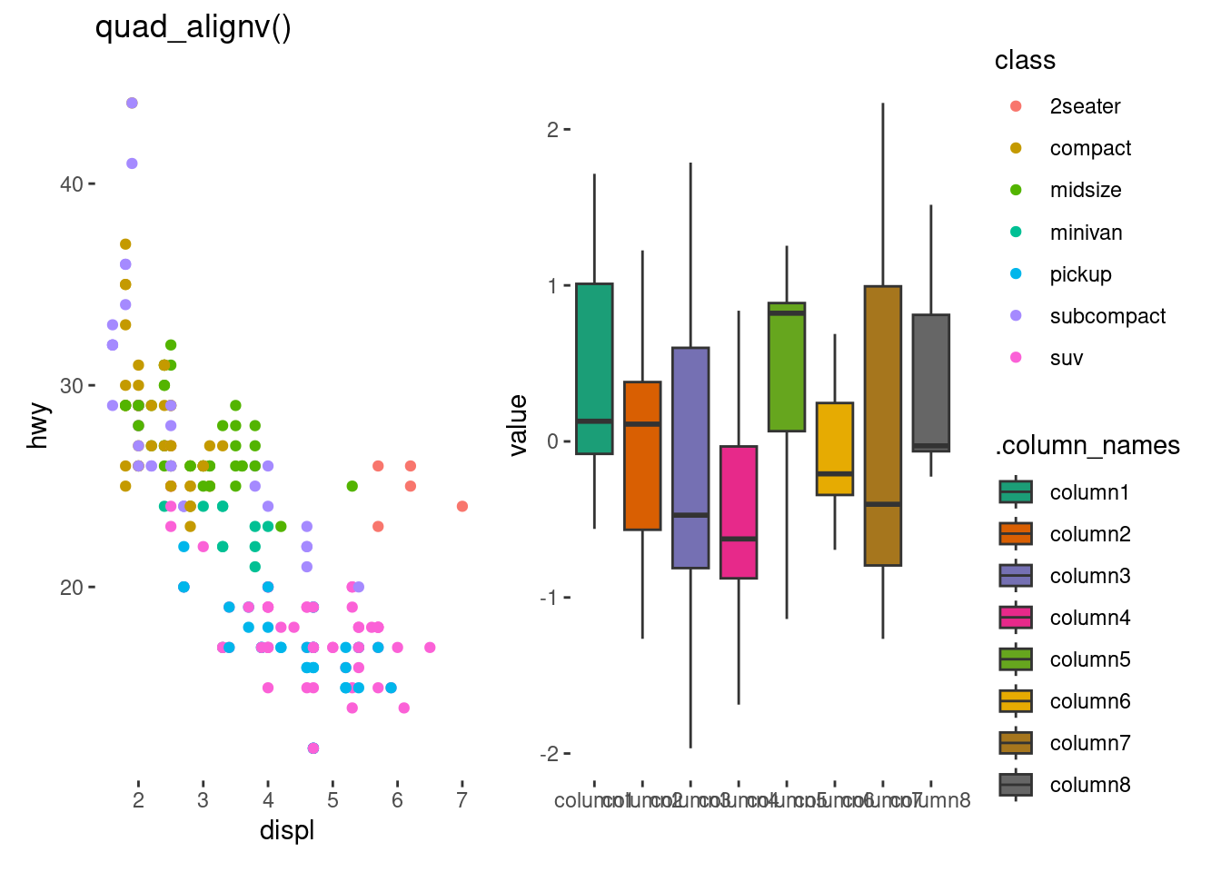

Alternatively, you can set initialize = TRUE, which will initialize the annotation stack layout with no data. In this case, you must provide data in each plot within the annotation.

quad_layout(small_mat, xlim = NULL) +
    geom_boxplot(aes(value, .discrete_y, fill = .row_names)) +
    scale_fill_brewer(palette = "Dark2") +
    anno_top(initialize = TRUE) +
    ggalign(data = mpg, aes(displ, hwy, colour = class)) +
    geom_point(aes(displ, hwy, colour = class))+
    layout_title("quad_alignh()")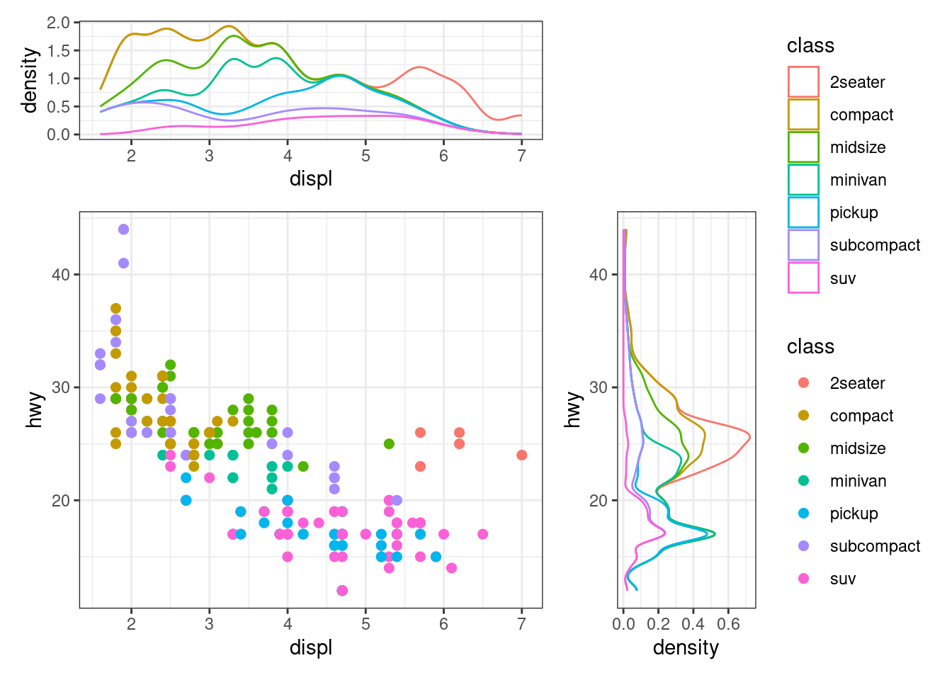

quad_layout(small_mat, ylim = NULL) +
    geom_boxplot(aes(.discrete_x, value, fill = .column_names)) +
    scale_fill_brewer(palette = "Dark2") +
    anno_left(initialize = TRUE) +
    ggalign(data = mpg, aes(displ, hwy, colour = class)) +
    geom_point(aes(displ, hwy, colour = class))+
    layout_title("quad_alignv()")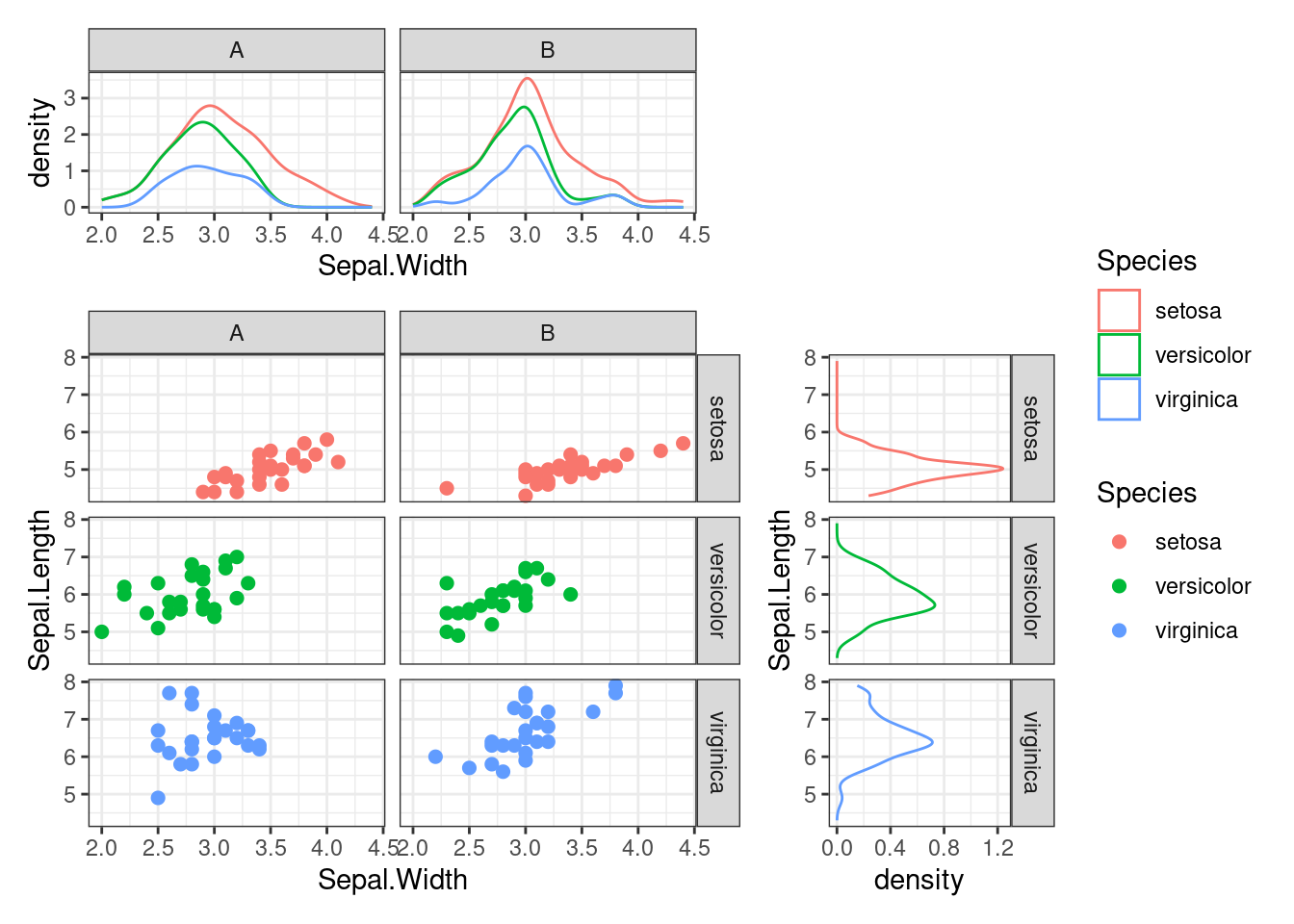

Now we have explored all the Layout defined in the package, there are something special for stack_layout() and quad_layout(), as you should already know quad_layout() can take stack_layout() as the input (Section 7.5), Similarly, stack_layout() can also accept a quad_layout() as input, which is particularly useful for arranging multiple quad_layout()/ggheatmap() objects together.

In the next chapter, we will explore even more advanced techniques for combining multiple quad_layout()s. These methods will provide you with the tools to manage more complex plot arrangements and make your visualizations even more flexible and powerful.