ggmark() can be used to add annotation plot for the selected observations. ggmark accepts mark argument, which should be a mark_draw() object to define how to draw the links.
Currently, two helper functions are provided to generate these links:
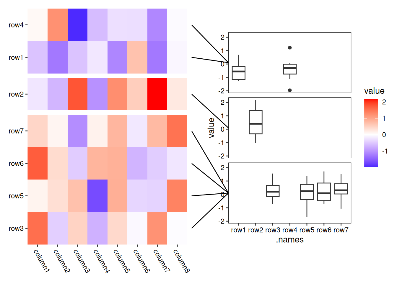
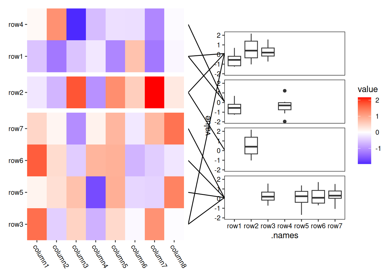
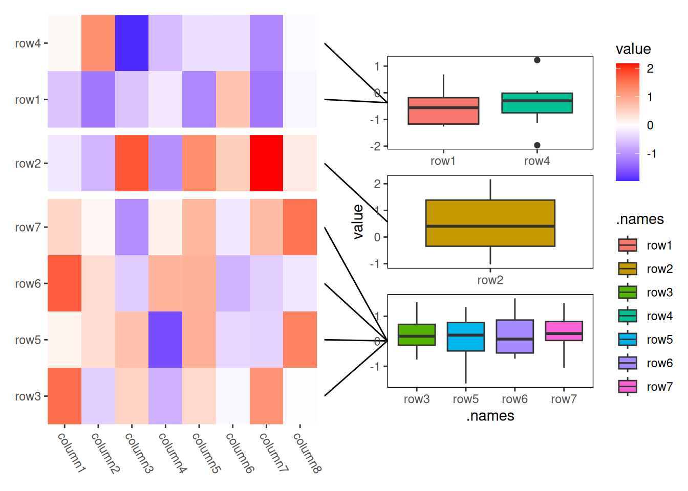
mark_line(): draws a line to the annotation panel.
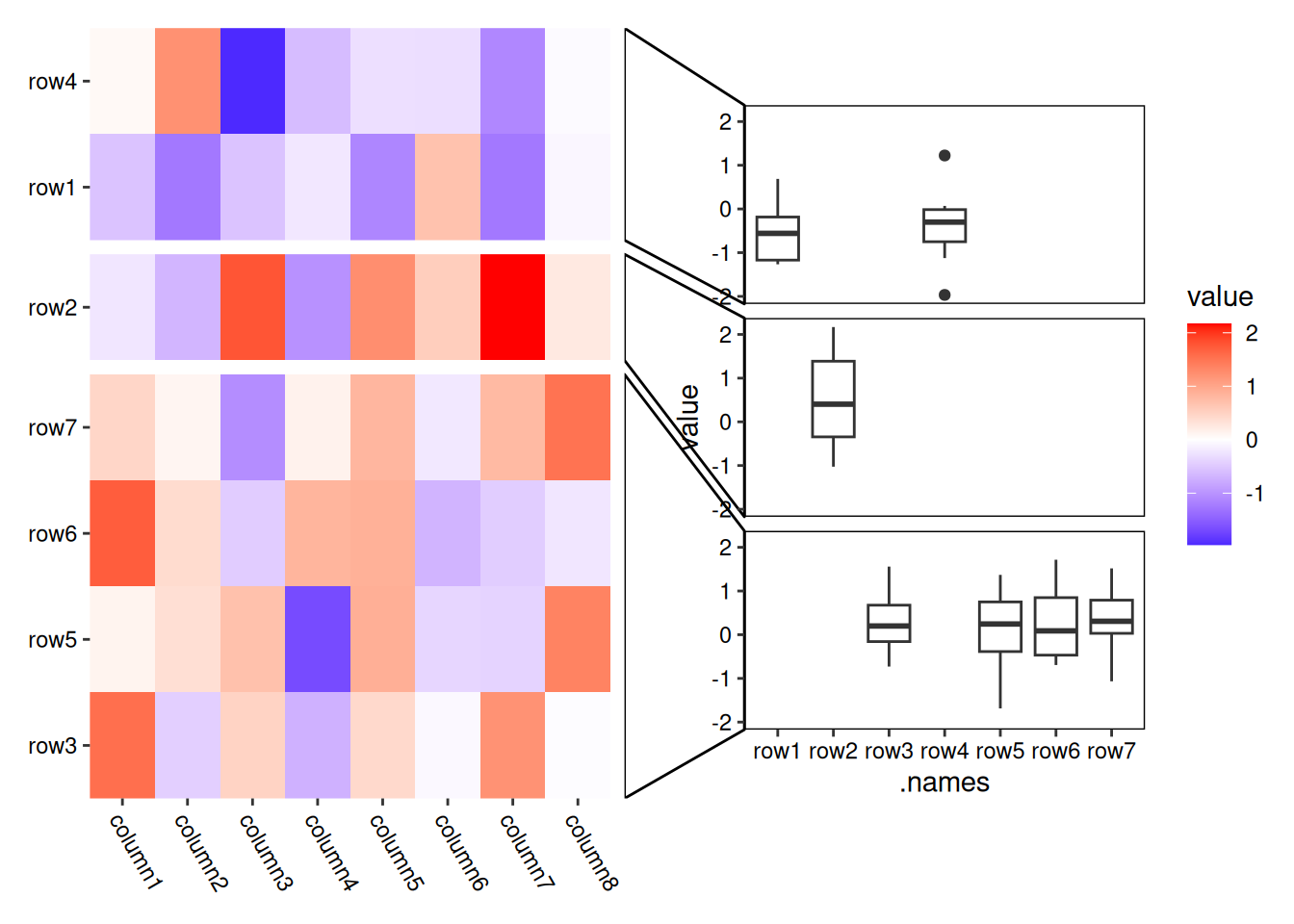
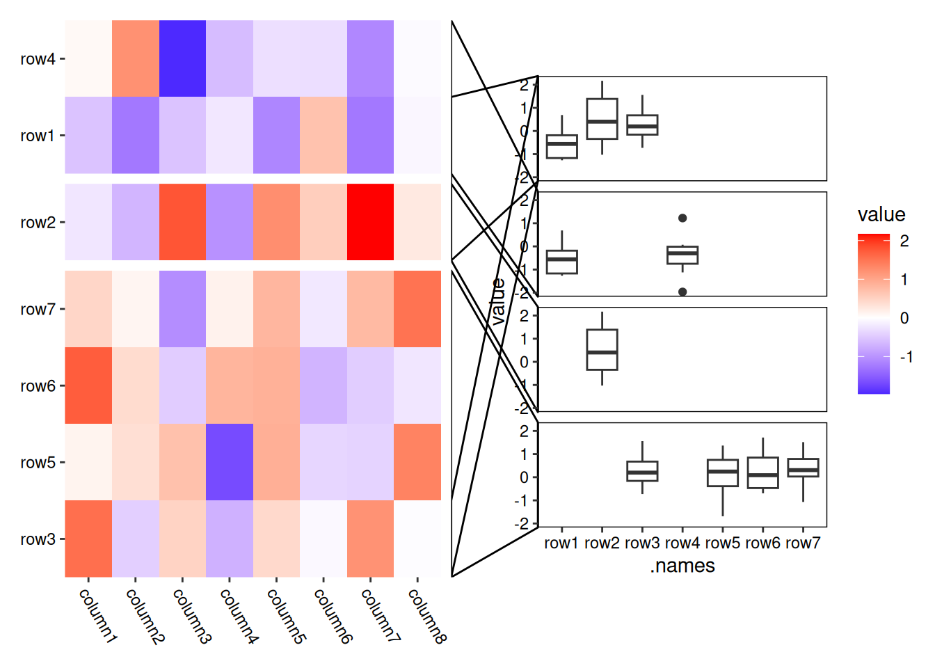
mark_tetragon(): draws a quadrilateral shape connecting observations and the panel.
All of these functions specify links as pair_links() as introduced in Chapter 15. Each pair of links will introduce a panel in ggmark to annotate these observations.
Code
library(ggalign)#> Loading required package: ggplot2#> ========================================#> ggalign version 1.2.0.9000#> #> If you use it in published research, please cite: #> Peng, Y.; Jiang, S.; Song, Y.; et al. ggalign: Bridging the Grammar of Graphics and Biological Multilayered Complexity. Advanced Science. 2025. doi:10.1002/advs.202507799#> ========================================set.seed(123)small_mat<-matrix(rnorm(56), nrow =7)rownames(small_mat)<-paste0("row", seq_len(nrow(small_mat)))colnames(small_mat)<-paste0("column", seq_len(ncol(small_mat)))
16.1 plot data
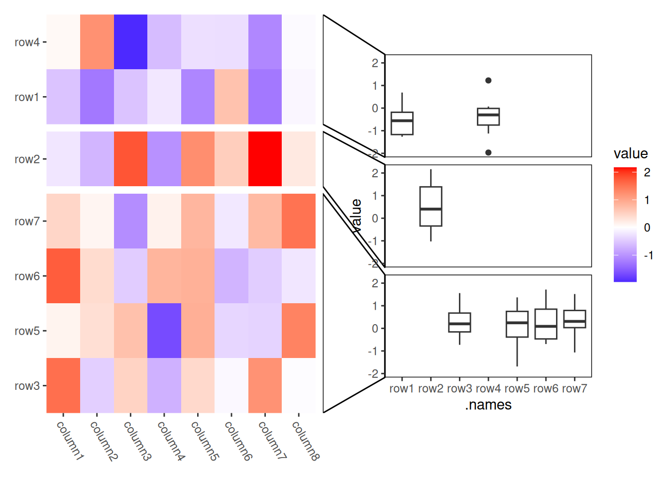
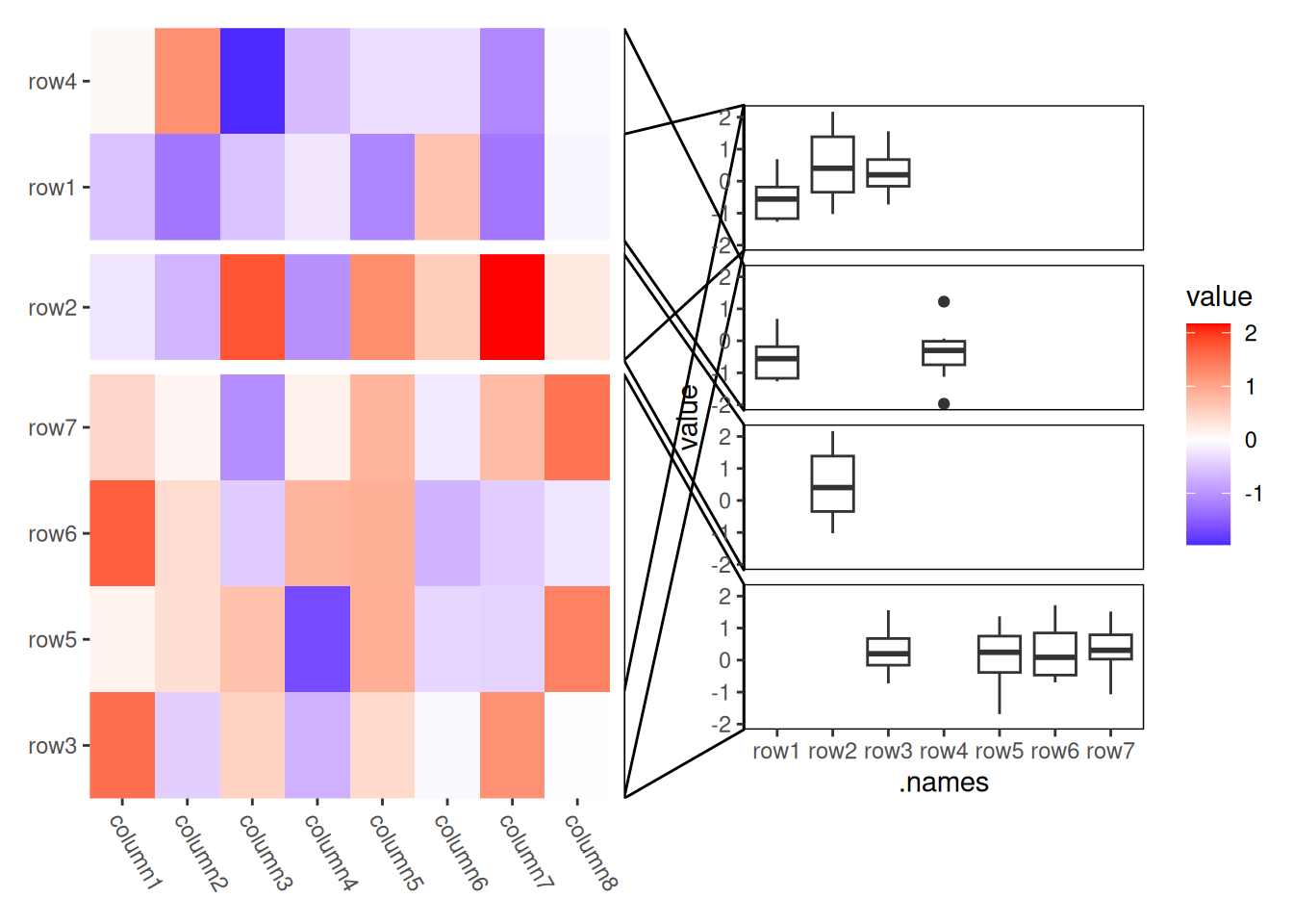
By default, if no observations are explicitly selected, ggmark() selects all observations and splits them based on the layout’s grouping.
Calling ggmark() initializes a ggplot object, the underlying data is created using fortify_data_frame(). Please refer to it for more details. In addition, the following columns will be added to the data frame:
.panel: the panel for the aligned axis. It means x-axis for vertical stack layout (including top and bottom annotation), y-axis for horizontal stack layout (including left and right annotation).
.names and .index: a character names (only applicable when names exists) and an integer of index of the original data.
.hand: A factor with levels c("left", "right") for horizontal stack layouts, or c("top", "bottom") for vertical stack layouts, indicating the position of the linked observations.
By default, ggmark() uses facet_wrap to define the facet, and you can use it to control the facet apearance (just ignore the facets argument). We prefer facet_wrap() here because it offers flexibility in positioning the strip on any side of the panel, and typically, we only want to a single dimension to create the annotate the selected observations. However, you can still use facet_grid() to create a two-dimensional plot. Note that for horizontal stack layouts, the row facets, or for vertical stack layouts, the column facets will always be overwritten.
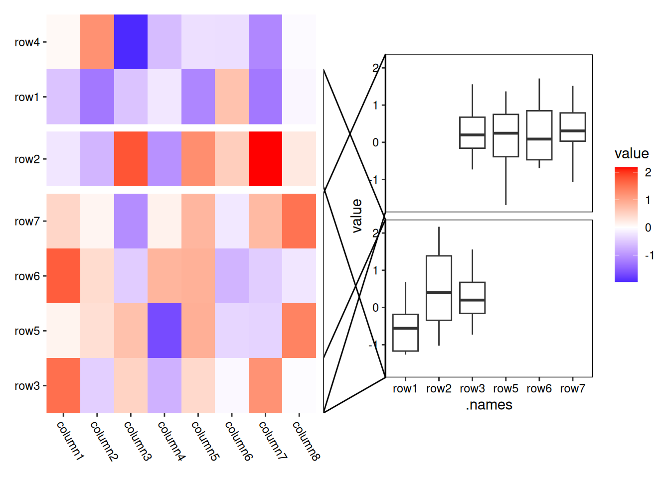
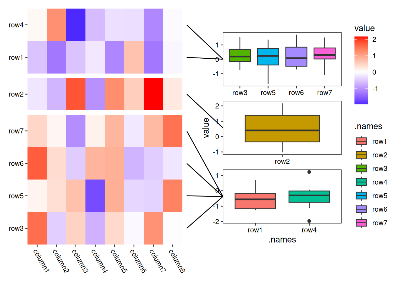
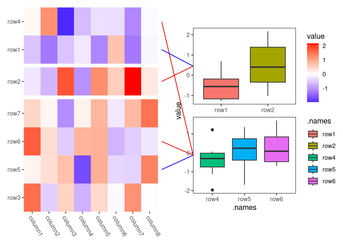
set.seed(123)ggheatmap(small_mat)+theme(axis.text.x =element_text(hjust =0, angle =-60))+anno_right()+align_kmeans(3L)+ggmark(mark_tetragon(4:6, 1:2, .element =element_polygon(fill =c("red", "blue"), alpha =0.5)))+geom_boxplot(aes(.names, value, fill =.names))+facet_wrap(vars(), scales ="free", strip.position ="right")+theme(plot.margin =margin(l =0.1, t =0.1, unit ="npc"))#> Warning in element_polygon(fill = c("red", "blue"), alpha = 0.5): `...` must be empty.#> ✖ Problematic argument:#> • alpha = 0.5#> → heatmap built with `geom_tile()`
You can wrap the element with I() to recycle it to match the drawing groups. The drawing groups typically correspond to the number of observations for element_line(), as each observation will be linked with the plot panel.
For element_polygon(), the drawing groups usually align with the defined groups. However, if the defined group of observations is separated and cannot be linked with a single quadrilateral, the number of drawing groups will be larger than the number of defined groups.
For stack_discrete(), we usually don’t need to specify both hands in the formula, since they are expected to share the same ordering and group structure. This is because all plots within stack_discrete() maintain a common ordering index across the layout.
However, explicitly specifying another hands becomes useful in stack_cross(), where different observation orderings are involved. This scenario is covered in (stack-cross?).
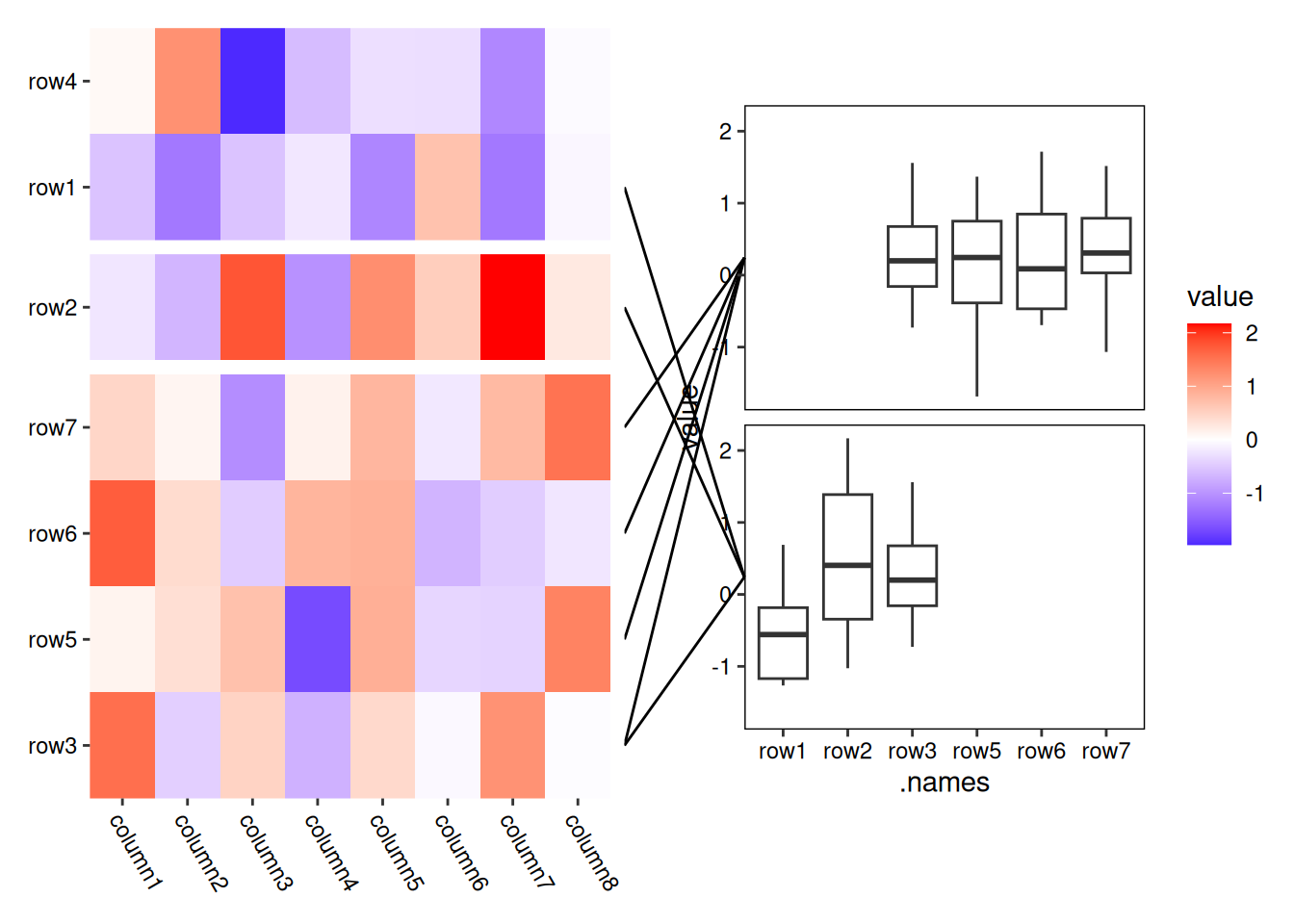
Both mark_line() and mark_tetragon() are built on top of mark_draw() (strictly, .mark_draw()). This function allows you to define custom mark styles by supplying a drawing function which must return a grob/gList.
The function passed to mark_draw() must accept two arguments:
A data frame representing the panel-side coordinates (ggmark plot)
A data frame representing the observation-side coordinates
Each observation is assumed to occupy a unit length in the layout. Therefore, the observation-side coordinates include two terminal points x, y, xend, yend—representing the start and end of the observation along the linking axis.
Additional columns in the link data frame include:
link_id: The identifier of the link (e.g., following example 4:6 link has id “a”).
link_panel: Indicates which panel the link is drawn to, based on the layout.
link_index: The layout index for positioning.
.hand: Either “left”/“right” (horizontal) or “top”/“bottom” (vertical), specifying the hand of the observation.
.index: The original index of the observation.
Here is an example that prints the structure of the panel and link data frames:
set.seed(123)p<-ggheatmap(small_mat)+theme(axis.text.x =element_text(hjust =0, angle =-60))+anno_right()+align_kmeans(3L)+ggmark(mark_draw(function(panel, link){print(panel)print(link)}, a =4:6, 1:2))pdf(NULL)print(p)#> → heatmap built with `geom_tile()`#> x xend y yend#> 1 0.02720374 0.02720374 0.01235571 0.4938221#> x xend y yend link_id link_panel link_index .hand .index#> 1 0 0 0.8606731 1.0000000 a 3 7 left 4#> 2 0 0 0.1393269 0.2786539 a 1 2 left 5#> 3 0 0 0.2786539 0.4179808 a 1 3 left 6#> x xend y yend#> 1 0.02720374 0.02720374 0.5061779 0.9876443#> x xend y yend link_id link_panel link_index .hand .index#> 1 0 0 0.7213461 0.8606731 2 3 6 left 1#> 2 0 0 0.5696635 0.7089904 2 2 5 left 2invisible(dev.off())
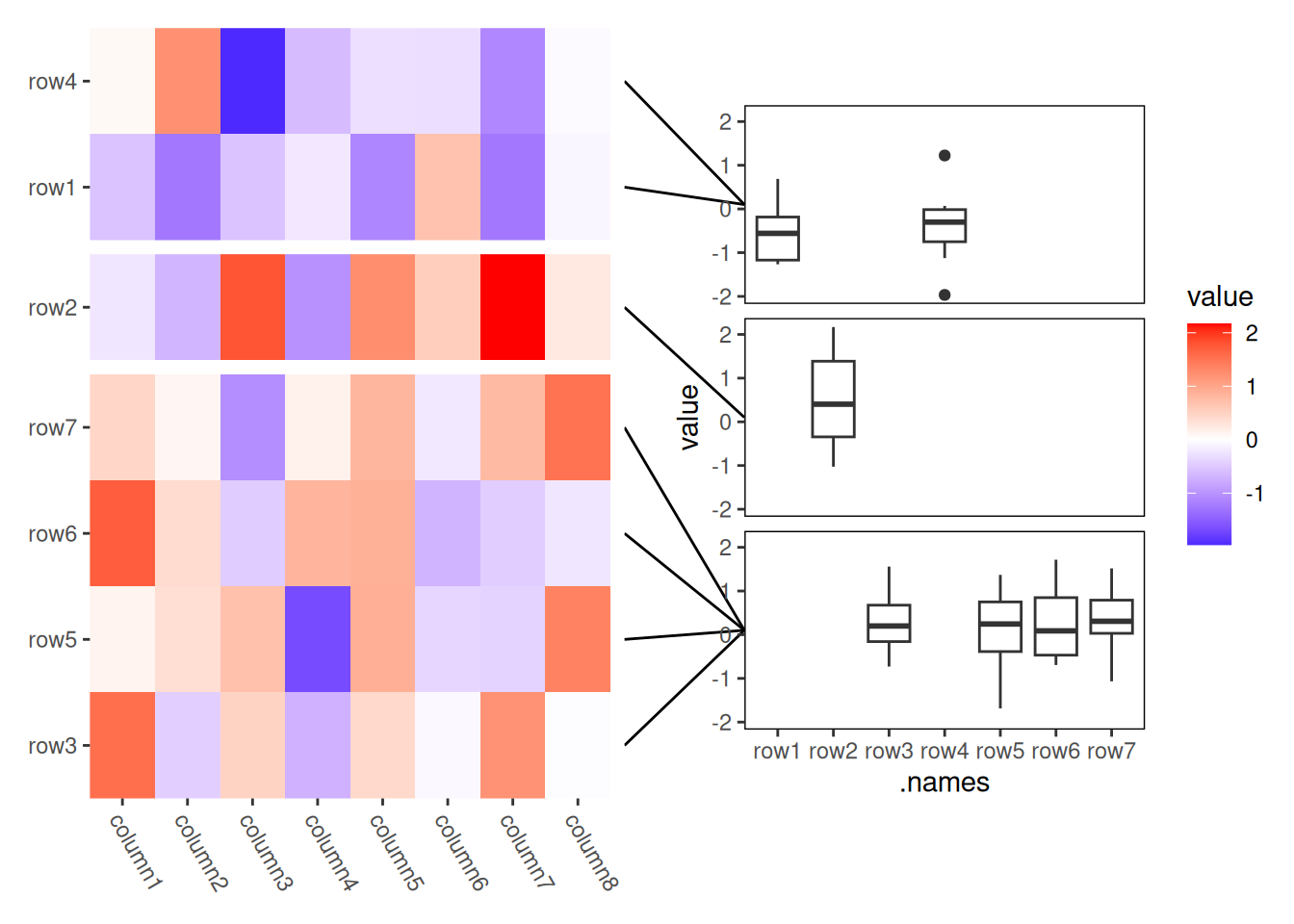
Here, we draw a triangle to connect the
set.seed(123)ggheatmap(small_mat)+theme(axis.text.x =element_text(hjust =0, angle =-60))+anno_right()+align_kmeans(3L)+ggmark(mark_draw(function(panel, link){x<-c((panel$x+panel$xend)/2L, link$x, link$xend)y<-c((panel$y+panel$yend)/2L, link$y, link$yend)grid::polygonGrob(x, y)}, 4, 2)# selecting one observation from each group for simple example)+geom_boxplot(aes(.names, value, fill =.names))+facet_wrap(vars(), scales ="free", strip.position ="right")+theme(plot.margin =margin(l =0.1, t =0.1, unit ="npc"))#> → heatmap built with `geom_tile()`