Code
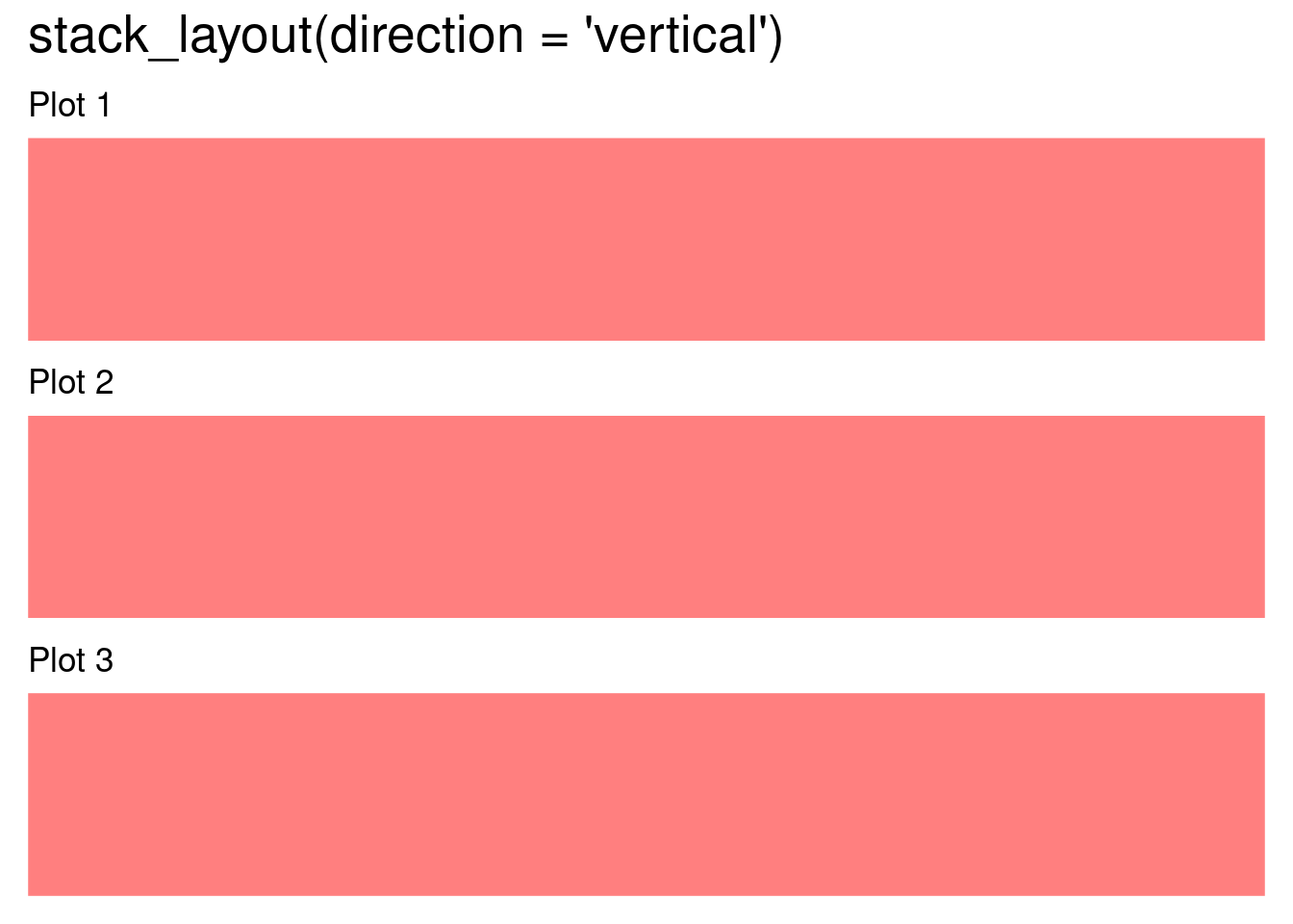
library(ggalign)stack_layout() arranges plots either horizontally or vertically. Based on whether we want to align the discrete or continuous variables, there are two types of stack layouts:
stack_discrete(): Align discrete variable along the stack.stack_continuous(): Align continuous variable along the stack.stack_layout() integrates the functionalities of stack_discrete() and stack_continuous() into a single interface. The first argument for these three functions is direction which should be a single string indicating the direction of the stack layout, either "h"(horizontal) or "v"(vertical).
Several aliases are available for convenience:
stack_discretev: A special case of stack_discrete that sets direction = "v".stack_discreteh: A special case of stack_discrete that sets direction = "h".stack_continuousv(): A special case of stack_continuous that sets direction = "v".stack_continuoush(): A special case of stack_continuous that sets direction = "h".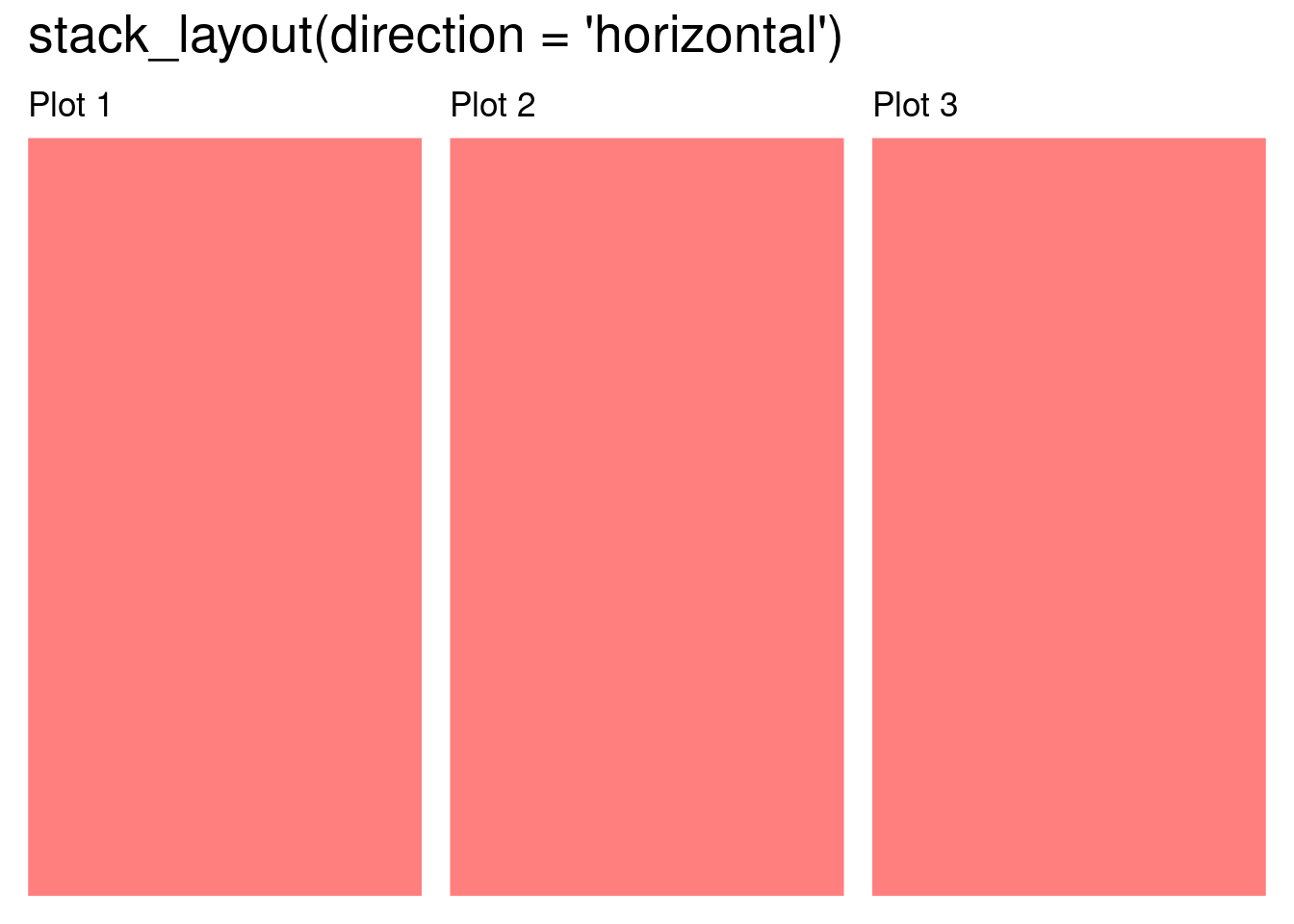
library(ggalign)As discussed in Section 5.3, when aligning discrete variables, we typically use a matrix. For continuous axes, we can still use the long-formatted data frame, which is the same as in ggplot2.
stack_continuous(), a data frame is required, and the input will be automatically converted using fortify_data_frame() if needed.stack_discrete(), a matrix is required, and the input will be automatically converted using fortify_matrix() if needed.set.seed(123)
small_mat <- matrix(rnorm(56), nrow = 7)
rownames(small_mat) <- paste0("row", seq_len(nrow(small_mat)))
colnames(small_mat) <- paste0("column", seq_len(ncol(small_mat)))stack_discrete()/stack_continuous() will set up the layout, but no plot will be drawn until you add a plot element:
stack_discretev(small_mat)
# the same for `stack_continuous()`![]()
The data input when initializing the layout will be regarded as the default data, which can be inherited by all plots added to the layout.
For stack_discrete(), when default data is provided, the number of observations (nobs) is determined by the number of rows in the input matrix (i.e., NROW()). All plots added to the layout must use data with the same nobs. If you do not provide default data when initializing the layout, the first element you add—if it includes data—will determine the layout’s nobs.
Without any plots, it’s difficult to see how each layout system works in practice. Here, we introduce the most common plot adding function-ggalign(). This function plays a role similar to ggplot2::ggplot() function-it initialize a ggplot object-but is designed specifically for use within the the Layout system of Data-Aware Composition.
When ggalign() is added to the layout, it inherits the layout data and sets itself as the active plot. This means any subsequent + operations will apply to that plot. You can add standard ggplot2 components like geoms, stats, scales, etc.
When aligning discrete variables, the underlying data passed to ggplot through ggalign() will include the following columns (more details will be introduced in Section 9.1):
.x/.y and .discrete_x/.discrete_y: an integer index of x/y coordinates and a factor of the data labels (only applicable when names/rownames exists)..names and .index: A character names (only applicable when names/rownames exists) and an integer of index of the original data.For horizontal stack, the y-axis is aligned-the rows correspond to the y-axis.
For vertical stack, the x-axis is aligned-the rows correspond to the x-axis.
You must use
.x/.y, or.discrete_x/.discrete_yas thex/yaesthetic mapping in order to enable axis alignment.
When rendering, the input data is matched to the layout data by row index.
As mentioned in Section 5.3, if the input is a matrix, it will be automatically converted into a long-formatted data frame (the meanings of the resulting columns match their names; see ?fortify_data_frame.matrix for details):
head(fortify_data_frame(small_mat))
#>   .row_index .column_index       value .row_names .column_names
#> 1          1             1 -0.56047565       row1       column1
#> 2          2             1 -0.23017749       row2       column1
#> 3          3             1  1.55870831       row3       column1
#> 4          4             1  0.07050839       row4       column1
#> 5          5             1  0.12928774       row5       column1
#> 6          6             1  1.71506499       row6       column1
Note the first argument of ggalign() is the data, so you must explicitly name the mapping argument.
stack_discretev(small_mat) +
    ggalign(mapping = aes(.x, value, fill = .discrete_x)) +
    geom_boxplot() +
    theme(axis.text.x = element_text())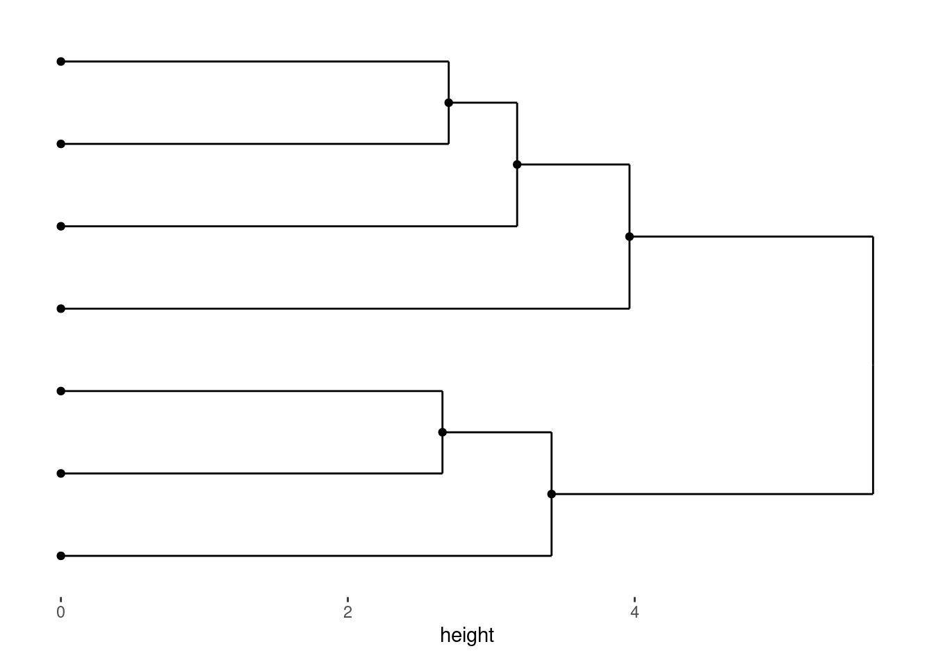
By default, axis text on the aligned axis (for vertical stack, x-axis) is removed to prevent duplicate labels. You can re-enable it using theme().
One major benefit of this system is that it supports algorithmic ordering of observations (note: rows are considered as observations, Section 9.1) and grouping observations into panels.
I’ll now introduce the most common algorithm — hierarchical clustering, which can also generate dendrograms: align_dendro() (more details will be introduced in Section 9.4). When you add align_dendro(), it can inherit the layout data, computes the dendrogram, and sets the global row ordering of the layout. It also creates a new ggplot object to draw the dendrogram.
stack_discretev(small_mat) +
    align_dendro() +
    ggalign(mapping = aes(.x, value, fill = .discrete_x)) +
    geom_boxplot() +
    theme(axis.text.x = element_text())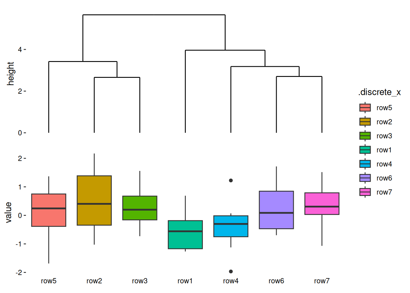
The main strength of ggalign is the alignment of discrete variables; continuous variable support is provided mainly for completeness. Here we show basic usage for aligning continuous variables.
stack_continuousv(mtcars) +
    ggalign(mapping = aes(mpg, disp, color = factor(cyl))) +
    geom_point() +
    theme(axis.text.x = element_text()) +
    ggalign(mapping = aes(mpg, hp, color = factor(cyl))) +
    geom_point() +
    theme(axis.text.x = element_text())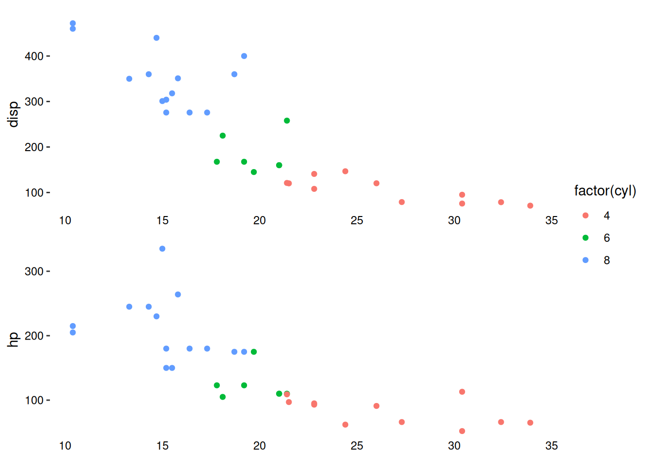
Similar to stack_discretev(), by default, axis text on the aligned axis (for vertical stacks, the x-axis) is removed to prevent duplicate labels. You can explicitly control visibility using theme().
In this example, no special alignment occurs because both ggalign() calls inherit the same default data, resulting in identical axis limits.
To demonstrate differences, here we filter the data to make the plot x-axis limits different. By default, stack_continuous() does not set axis limits:
stack_continuousv(mtcars) +
    ggalign(mapping = aes(mpg, disp, color = factor(cyl))) +
    geom_point() +
    theme(axis.text.x = element_text()) +
    ggalign(
        ~ dplyr::filter(.x, mpg < 20),
        mapping = aes(mpg, hp, color = factor(cyl))
    ) +
    geom_point() +
    theme(axis.text.x = element_text())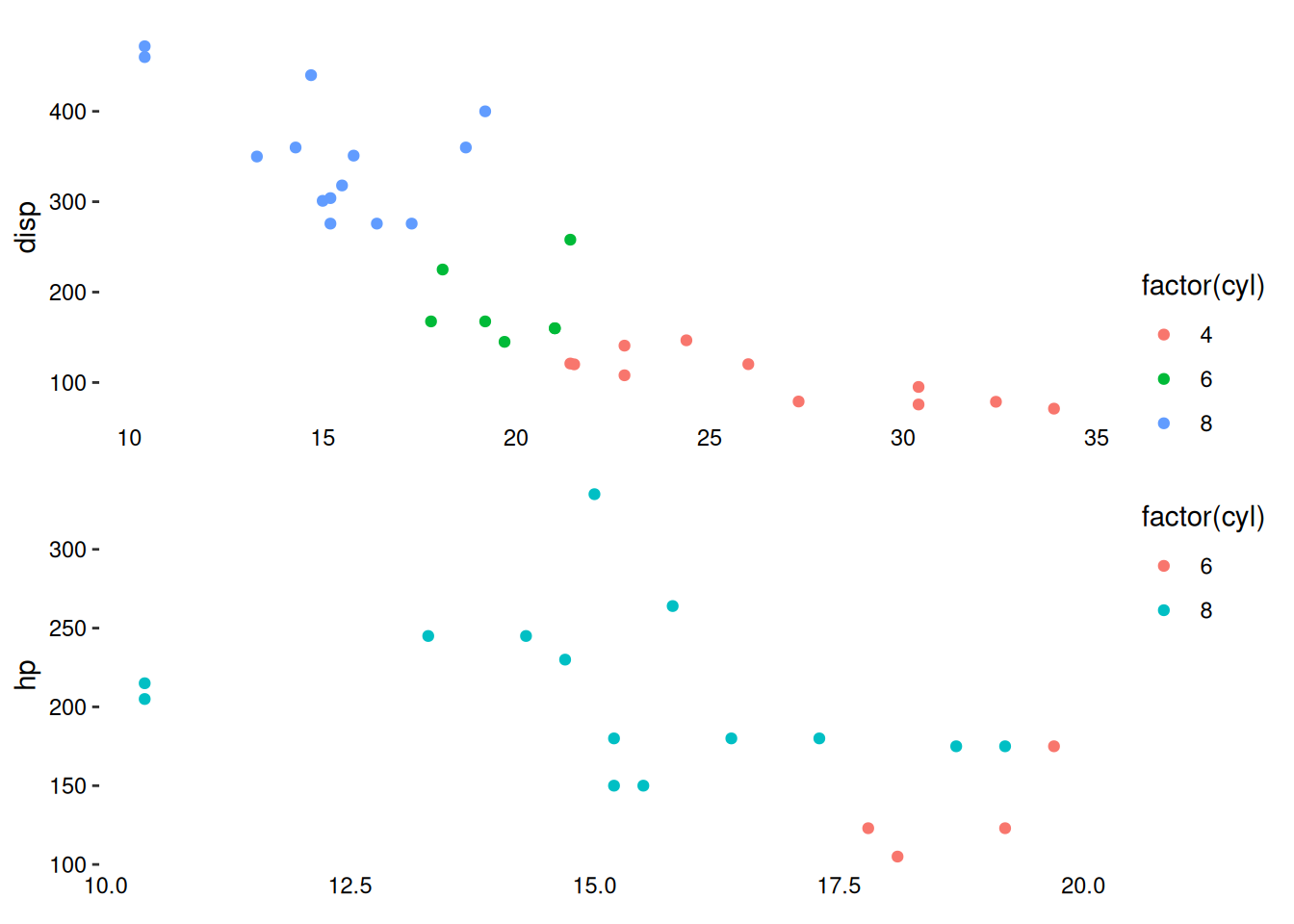
To align the x-axis limits, you must manually set them using the limits argument, which accepts a continuous_limits() object. continuous_limits() takes a numeric vector of length 2, defining the axis limits for each panel along the aligned axis.
The data argument in ggalign can be a purrr-style function that transforms the default data and returns new data.
stack_continuousv(mtcars, limits = continuous_limits(c(NA, 20))) +
    ggalign(mapping = aes(mpg, disp, color = factor(cyl))) +
    geom_point() +
    theme(axis.text.x = element_text()) +
    ggalign(~ dplyr::filter(.x, mpg < 20), mapping = aes(mpg, hp, color = factor(cyl))) +
    geom_point() +
    theme(axis.text.x = element_text())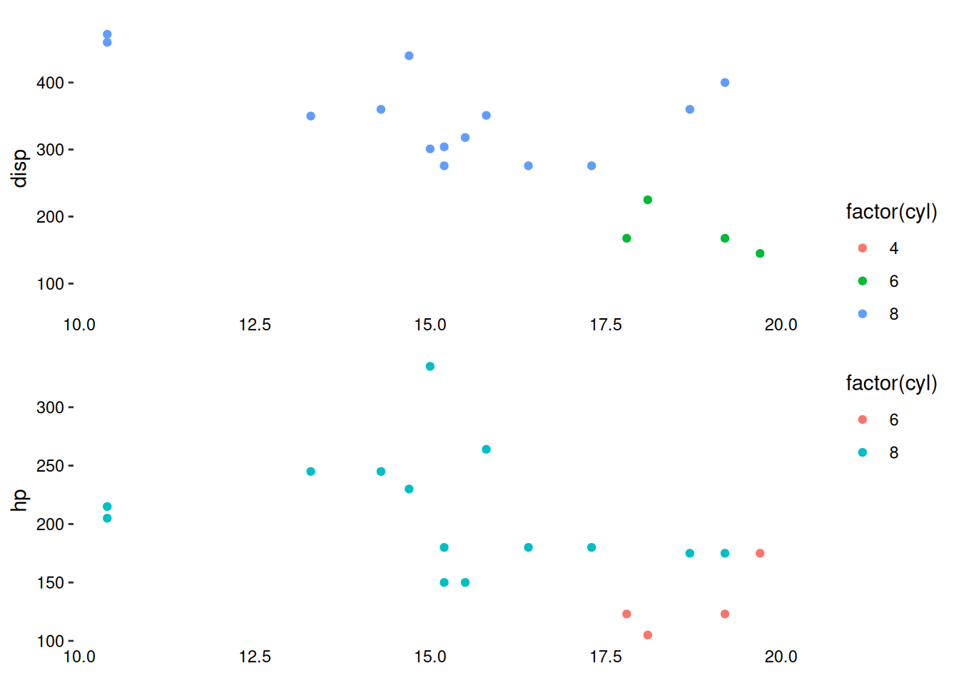
Aside from differences in input data, most operations in stack_discrete() also apply to stack_continuous(). The key distinction lies in how alignment is handled, as discussed in Section 5.3: stack_continuous() does not support the Layout customization system used for discrete variables.
Because of this, we will focus on stack_discrete(). Nearly all techniques shown can also be used with stack_continuous(), except for Layout customization.
All plot adding functions have a size argument to control the relative width (for horizontal stack layout) or height (for vertical stack layout) of the plot’s panel area.
stack_discretev(small_mat) +
    align_dendro(size = 1) +
    ggalign(mapping = aes(.x, value, fill = .discrete_x), size = 2) +
    geom_boxplot() +
    theme(axis.text.x = element_text())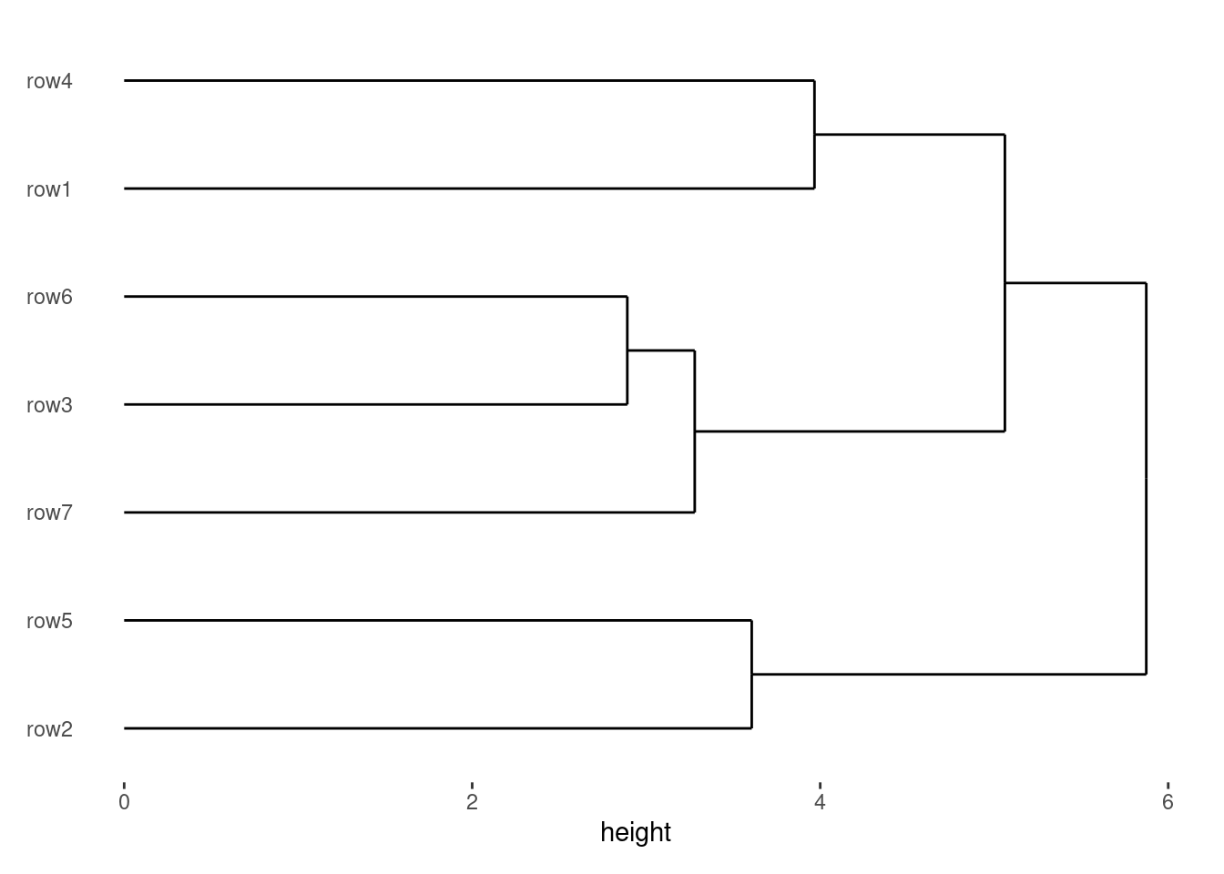
Alternatively, you can define an absolute size by using a unit() object:
stack_discretev(small_mat) +
    align_dendro(size = unit(1, "cm")) +
    ggalign(mapping = aes(.x, value, fill = .discrete_x), size = 2) +
    geom_boxplot() +
    theme(axis.text.x = element_text())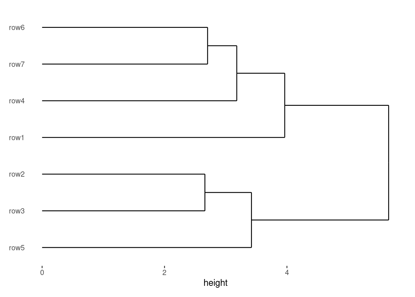
In the next chapter, we will dive into the HeatmapLayout, which can take the StackLayout as input. Heatmap layouts offer additional features for aligning observations in both directions. Let’s move ahead and explore how heatmaps can be seamlessly integrated into your layout workflows.