3  Plot Composer

The align_plots() function is the core engine for data-free composition in the ggalign package. It enables users to arrange multiple plots and graphical objects into a structured layout, with fine control over spacing, alignment, size, and guide collection — all independent of the underlying data or coordinate systems.

This section provides a comprehensive breakdown of its key arguments, along with how they affect the final layout.

Code
library(ggalign)
#> Loading required package: ggplot2
#> 
#> Attaching package: 'ggalign'
#> The following object is masked from 'package:ggplot2':
#> 
#>     element_polygon

We’ll start with a few well-known example plots:

p1 <- ggplot(mtcars) +
    geom_point(aes(mpg, disp))
p2 <- ggplot(mtcars) +
    geom_boxplot(aes(gear, disp, group = gear))
p3 <- ggplot(mtcars) +
    geom_bar(aes(gear)) +
    facet_wrap(~cyl)
p4 <- ggplot(mtcars) +
    geom_bar(aes(carb))
p5 <- ggplot(mtcars) +
    geom_violin(aes(cyl, mpg, group = cyl))

3.1 Plots Arrangement

You can pass plots as individual arguments:

align_plots(p1, p2, p3, p4, p5)

Or use bang-bang-bang to add a list of plots

align_plots(!!!list(p1, p2, p3), p4, p5)

3.2 Grid Layout

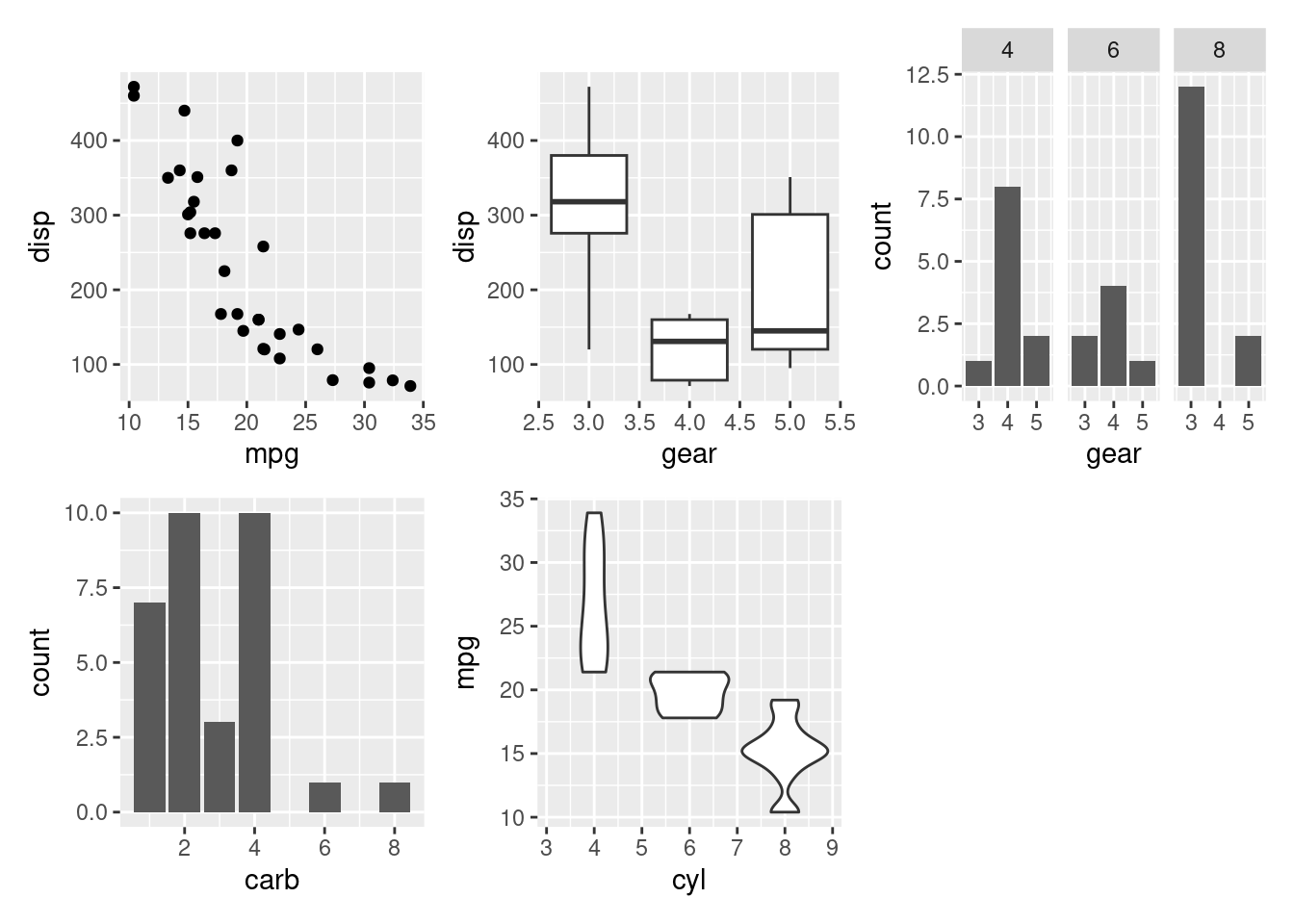
Like patchwork, if no specific layout is provided, align_plots() will attempt to create a grid that is as square as possible, with each column and row taking up equal space:

align_plots(p1, p2, p3, p4, ncol = 3)

Use byrow = FALSE to fill the grid column-wise (top to bottom, then left to right) instead of the default row-wise layout:

align_plots(p1, p2, p3, p4, p5, ncol = 3, byrow = FALSE)

Alternatively, use named layout strings for complex control over placement:

align_plots(
    A = p1, B = p2, C = p3,
    area = "
    AABB
    CCDD
  "
)

For even more control, you can use area() to define a layout manually:

align_plots(p1, p2, p3, p4, area = c(
    area(1, 1, 1, 2), # p1: spans columns 1–2
    area(2, 1, 3, 1), # p2: spans rows 2–3, column 1
    area(2, 2, 3, 2), # p3: same shape as p2, column 2
    area(4, 1, 4, 2) # p4: same shape as p1, row 4
))

3.3 Plot Panel Size

Use widths and heights to control how much space each panel column or panel row should take, respectively. These can be:

  • Relative values (e.g., widths = c(2, 1) means the first column is twice as wide)

  • unit() values from the grid package, if you want fixed sizing.

align_plots(p1, p2, p3, p4, widths = c(2, 1))

3.4 Leaving Empty Spaces

To create gaps in your layout, insert NULL where a plot would go:

align_plots(p1, NULL, p2, NULL, p3, NULL)

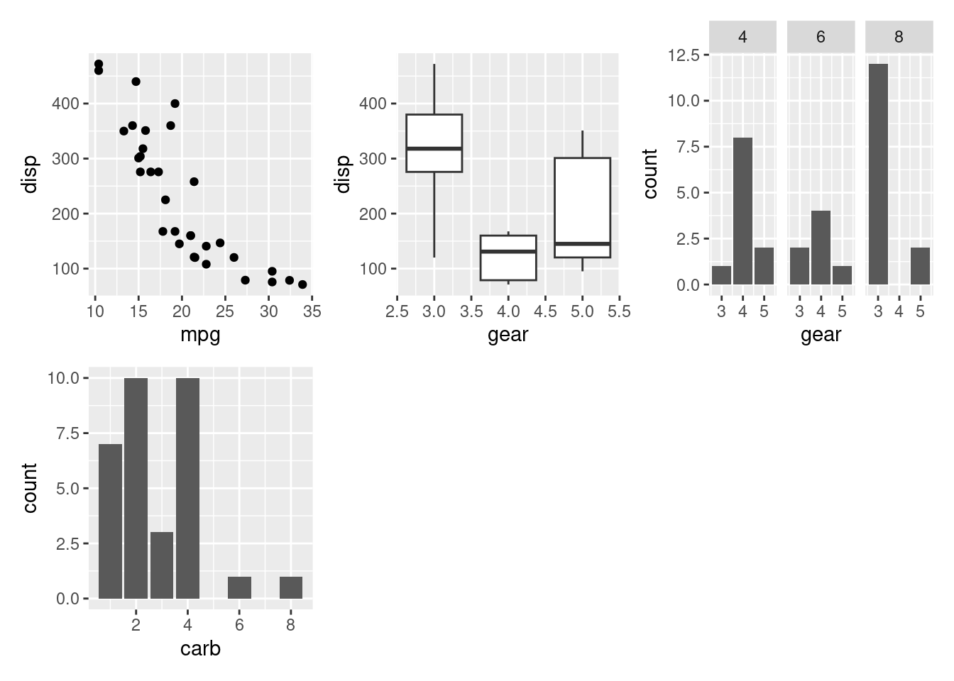
Empty cells will still take up layout space unless you explicitly adjust sizes.

3.5 Guide Legends

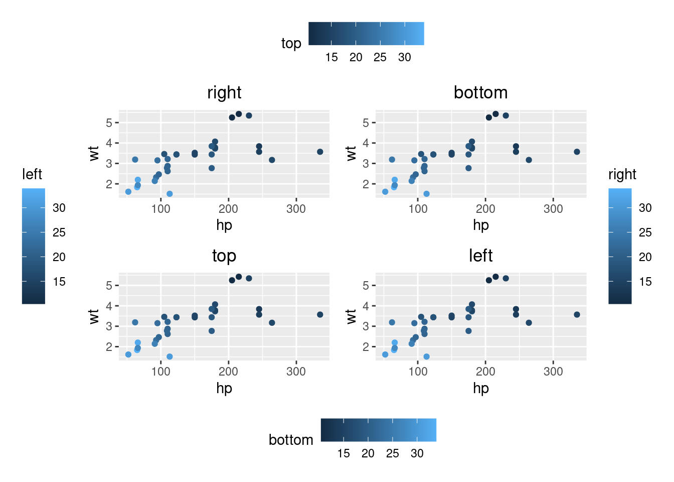
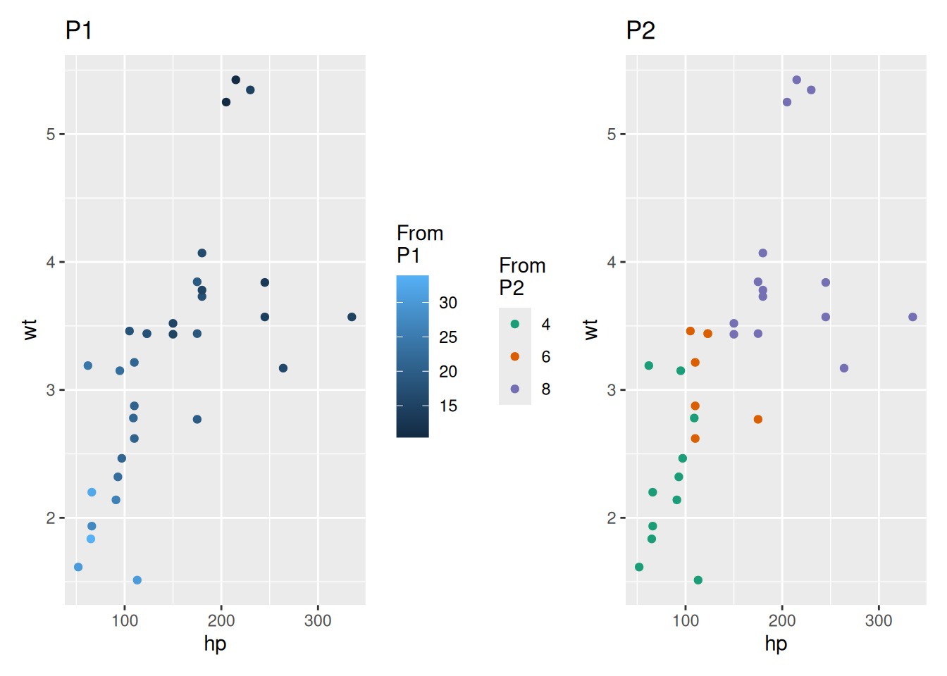
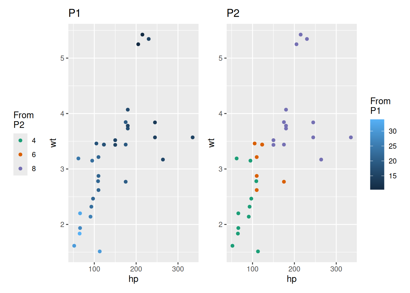
By default, each plot keeps its own guides. Use the guides argument to collect and consolidate them to specific sides, which should be of a single string with following elements:

  • "t" — collect top guide legends

  • "r" — collect right guide legends

  • "b" — collect bottom guide legends

  • "l" — collect left guide legends

  • "i" - Collect guide legends inside the plot panel area (plot panel guides)

p_right <- ggplot(mtcars) +
    geom_point(aes(hp, wt, colour = mpg)) +
    scale_color_continuous(guide = guide_colorbar(position = "right")) +
    labs(color = "From\nP1") +
    ggtitle("P1")

p_left <- ggplot(mtcars) +
    geom_point(aes(hp, wt, colour = factor(cyl))) +
    scale_color_brewer(
        palette = "Dark2",
        guide = guide_legend(position = "left")
    ) +
    labs(color = "From\nP2") +
    ggtitle("P2")
align_plots(p_right, p_left)

align_plots(p_right, p_left, guides = "lr")

If align_plots() is nested in another align_plots(), the nested align_plots() will inherit the guides argument from the upper-level align_plots(). And the top-level align_plots() won’t collect guide legends from plots within the nested align_plots() unless the nested align_plots() collects them first.