7 Heatmap Layout
The heatmap_layout() function provides a powerful way to create customizable heatmaps using ggplot2. This chapter will guide you through its usage.
heatmap_layout() is a specialized version of quad_discrete(), designed to align discrete variables both horizontally and vertically. We introduce heatmap_layout() directly, as it is more familiar to many users, especially those experienced with popular heatmap packages like pheatmap and ComplexHeatmap.
heatmap_layout() simplifies the creation of heatmap plots by integrating essential elements for a standard heatmap layout, ensuring that the appropriate data mapping and visualization layers are automatically applied. ggheatmap() is an alias for heatmap_layout().
7.1 Input Data
As mentioned in Section 5.3, we typically require a matrix for the Layout which need align discrete variables. Internally, fortify_matrix() will be used to process the data. You can provide a numeric or character vector, a data frame, or any other data type that can be converted into a matrix using as.matrix().
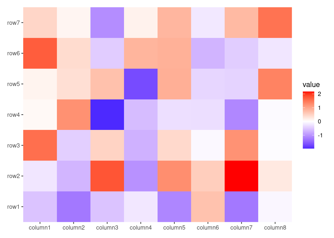
ggheatmap(small_mat)
#> → heatmap built with `geom_tile()`
7.2 Main Plot (Heatmap Body)
The ggheatmap()/quad_layout() functions arrange plots in the Quad-Side layout of the main plot. When the layout is initialized, a ggplot object is automatically created for the main plot.
For ggheatmap(), the matrix input will be converted into a long-format data frame when drawing. The data in the underlying ggplot object includes the following columns:
.xpaneland.ypanel: the column and row panel.xand.y: thexandycoordinates.row_namesand.column_names: A factor of the row and column names of the original matrix (only applicable when names exist)..row_indexand.column_index: the row and column index of the original matrix.value: the actual matrix value.
The default mapping will use aes(.data$.x, .data$.y), but can be customized using mapping argument.
By default, the main plot is regarded as the active plot, meaning you can add ggplot2 elements directly to the main plot.
ggheatmap(small_mat) +
    geom_point() +
    scale_fill_viridis_c()
#> → heatmap built with `geom_tile()`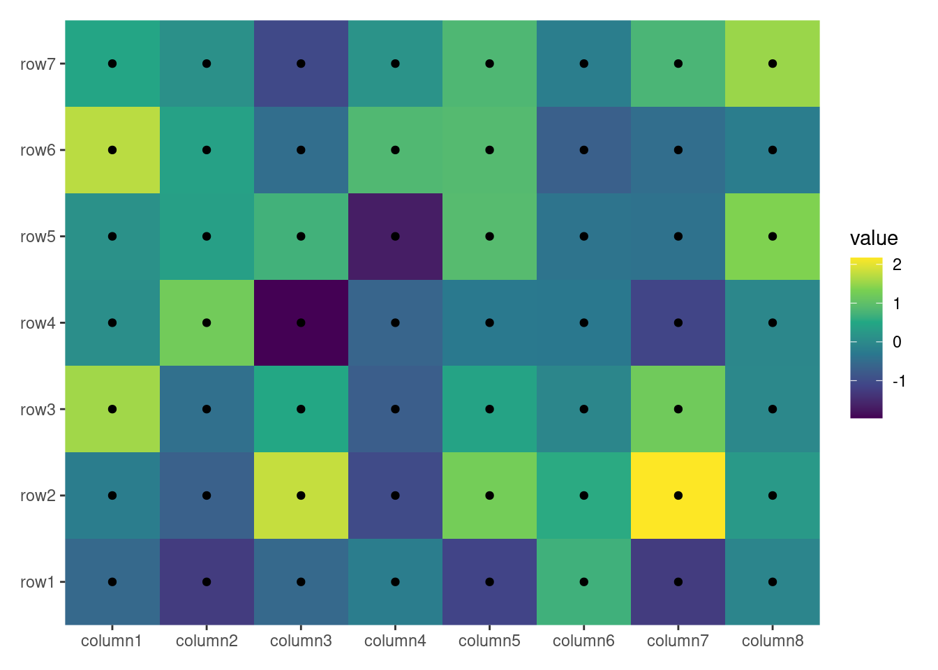
By default, ggheatmap() adds a heatmap layer. If the matrix has more than 20,000 cells (nrow * ncol > 20000), it uses geom_raster() for performance efficiency; for smaller matrices, geom_tile() is used. You can explicitly choose the layer by providing a single string ("raster" or "tile") in the filling argument.
ggheatmap(small_mat, filling = "raster")
ggheatmap(small_mat, filling = "tile")
Note, the filling layer will always use mapping of aes(.data$.x, .data$.y), if you want to customize filling, you can set filling = NULL, which will remove the filling layer and allow you to add custom filling geoms.

A heatmap pie charts can be easily drawn:
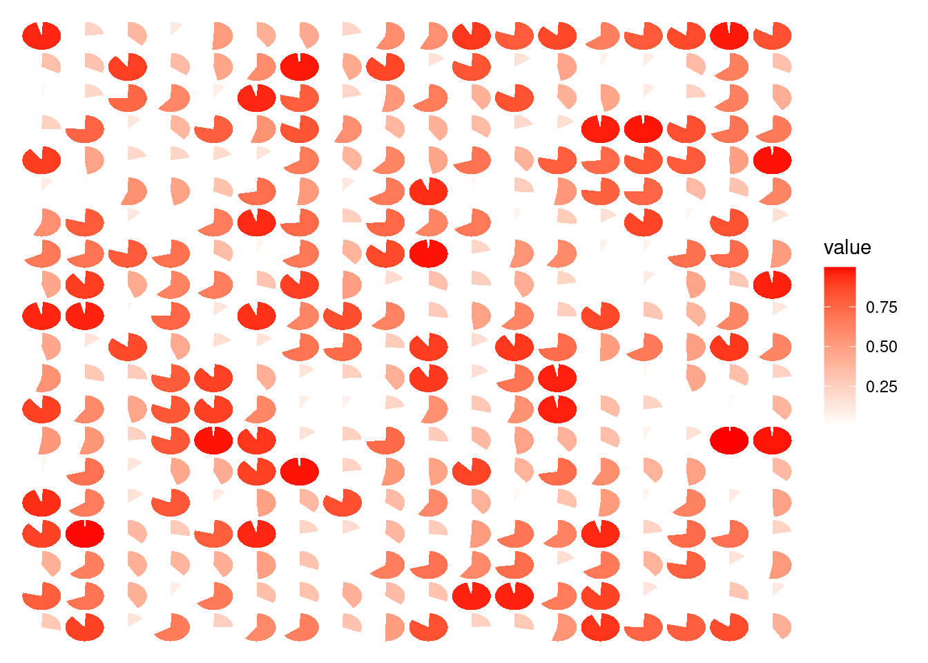
For more complex customizations of pie charts, you can try using ggforce::geom_arc_bar() instead.
7.3 Rasterization
When working with large heatmaps, it’s often beneficial to rasterize the heatmap body layer. You can achieve this by using the raster_magick() function. The res argument controls the resolution of the raster image. By default, the res argument matches the resolution of the current device, but specifying a different value can help reduce the resolution of the rasterized heatmap body.
ggheatmap(small_mat, aes(.x, .y), filling = NULL) +
    raster_magick(geom_tile(aes(fill = value)), res = 50)
By leveraging raster_magick(), you can also perform image post-processing using the magick package. This allows for custom image resizing with filters.
ggheatmap(small_mat, filling = NULL) +
    # Use `magick::filter_types()` to check available `filter` arguments
    raster_magick(geom_raster(aes(fill = value)),
        magick = function(image) {
            magick::image_resize(image,
                # we resize to the 50% of width
                geometry = "50%x", filter = "Lanczos"
            )
        }
    )
Note: When using magick::image_resize(), you should specify the geometry argument to resize the image. If only the filter is specified, it will only distort the image data (though subtle). For more information on image resizing, refer to ImageMagick’s resize documentation.
You can also rasterize all plots in the layout directly with raster_magick(). This method is defined for both ggheatmap()/quad_layout() and stack_layout() objects.
Additionally, You can use external packages like ggrastr or ggfx to rasterize the heatmap body.

Likewise, you can also rasterize all plots in the layout directly with ggrastr::rasterise() for both ggheatmap()/quad_layout() and stack_layout().
Furthermore, ggfx offers many image filters that can be applied to ggplot2 layers. See the package for the details.
7.4 Annotations
In ggheatmap()/quad_layout(), annotations are handled by a stack_layout() object and can be positioned at the top, left, bottom, or right of the main plot (heatmap body). quad_layout() can align discrete or continuous variables either horizontally or vertically. Since the annotation handling is the same for both ggheatmap() and quad_layout(), we introduce the annotation functionality for both together.
The annotations will always follow the alignment of the ggheatmap()/quad_layout() in the current direction. For horizontal alignment of discrete variables, stack_discreteh() will be used for left and right annotations, while stack_continuoush() will be used for continuous variables. The same logic applies to vertical alignment—stack_discretev() or stack_continuousv() will be used for top and bottom annotations, depending on whether the variables being aligned are discrete or continuous.
By default, ggheatmap()/quad_layout() do not activate an annotation, You can use quad_anno() to activate an annotation, directing all subsequent additions to the specified annotation position. The quad_anno() function has the following aliases:
-
anno_top: A special case ofquad_anno()withposition = "top". -
anno_left: A special case ofquad_anno()withposition = "left". -
anno_bottom: A special case ofquad_anno()withposition = "bottom". -
anno_right: A special case ofquad_anno()withposition = "right".
When quad_anno() is added to a ggheatmap()/quad_layout(), it will try to create a new stack_layout(). For top and bottom annotations, stack_discretev() or stack_continuousv() will be used; for left and right annotations, stack_discreteh() or stack_continuoush() will be applied.
Additionally, quad_anno() will set the active context to the annotation. This means that subsequent additions will be directed to the annotation rather than the main plot. We use the term active context in contrast to active plot (as discussed in Chapter 6), since the annotation is a Layout object but not a single plot.
ggheatmap(small_mat) +
    theme(axis.text.x = element_text(angle = -60, hjust = 0)) +
    anno_left() +
    align_dendro()
#> → heatmap built with `geom_tile()`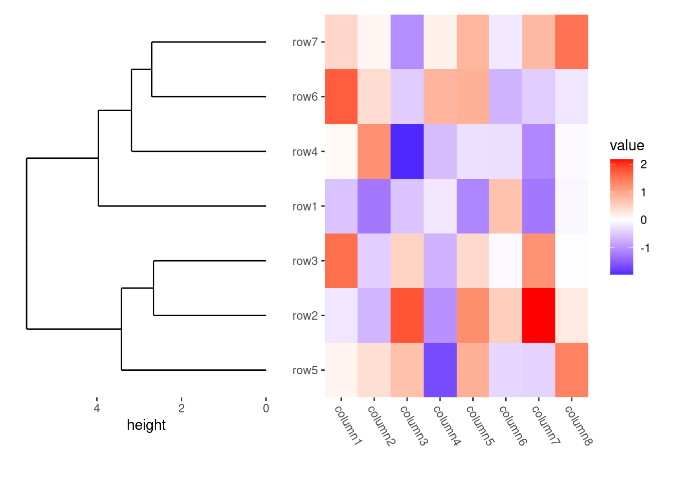
By default, the annotation stack_layout() attempts to inherit data from ggheatmap() or quad_layout(). When aligning discrete variables vertically, the data provided to ggheatmap() or quad_layout() must be a matrix. In this case, column annotations must also be based on a matrix. Internally, the matrix from ggheatmap() or quad_layout() will be transposed for use in column annotations, since rows are always treated as observations and alignment is performed along matrix rows.
ggheatmap(small_mat) +
    # we set the active context to the top annotation
    anno_top() +
    align_dendro()
#> → heatmap built with `geom_tile()`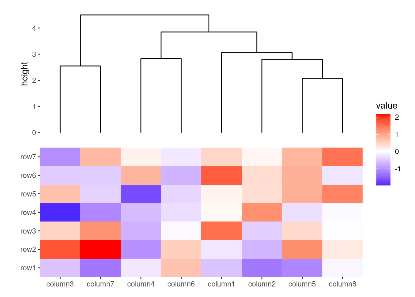
You can further customize the layout design or add new plots in the annotation stack, as described in Chapter 6.
ggheatmap(small_mat) +
    # in the heatmap body, we set the axis text theme
    theme(axis.text.x = element_text(angle = -60, hjust = 0)) +
    # we set the active context to the right annotation
    anno_right() +
    # in the right annotation, we add a dendrogram
    align_dendro(k = 3L) +
    # in the dendrogram, we add a point layer
    geom_point(aes(color = branch))
#> → heatmap built with `geom_tile()`
In this example:
-
anno_right()initialize the right annotation stack, and change the active context to the right annotation of the heatmap. -
align_dendro(k = 3L)adds a dendrogram to the annotation and sets itself as the active plot in the annotation stack. -
geom_point(aes(color = branch))is then added to this active plot within the annotation stack, here, it means thealign_dendro()plot.
Note: I’ll cover
align_dendro()in more detail in a later chapter. For now, just know that when you specify thekargument, the resulting internal data will include a branch column representing cluster assignments.
ggheatmap() aligns discrete variable both horizontally and vertically, so it’s safe to always use quad_anno() directly, as all annotations require a matrix, and the layout data is also a matrix. However, for quad_layout(xlim = NULL) and quad_layout(ylim = NULL) (which I’ll discuss in more detail in a Chapter 11), which only align discrete variable in one direction, the data in the layout may not fit the data for the annotation.
- `quad_layout(xlim = NULL)`: aligning discrete variable in horizontal
direction, for column annotations, we ll need a data frame for
`stack_continuous()`.
- `quad_layout(ylim = NULL)`: aligning discrete variable in vertical
direction, for row annotations, we ll need a data frame for
`stack_continuous()`.
In both cases, quad_anno() won’t initialize the annotation by default, instead, you must provide the annotation manually.
7.5 Adding Stack Layout
To add a stack_layout() to the ggheatmap(), we must prevent the automatic creation of annotations by quad_anno() by setting initialize = FALSE.
my_stack <- stack_discreteh(small_mat) +
    align_dendro(aes(color = branch), k = 3L)
ggheatmap(small_mat) +
    theme(axis.text.x = element_text(angle = -60, hjust = 0)) +
    anno_right(initialize = FALSE) +
    my_stack
#> → heatmap built with `geom_tile()`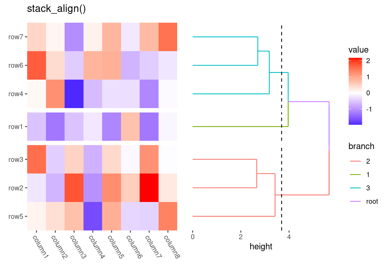
Note when aligning the discrete variable, you must ensure the number of observations is consistent in the direction. So for column annotations, you need transpose the data manually.
my_stack <- stack_discretev(t(small_mat)) +
    align_dendro(aes(color = branch), k = 3L)
ggheatmap(small_mat) +
    anno_top(initialize = FALSE) +
    my_stack
#> → heatmap built with `geom_tile()`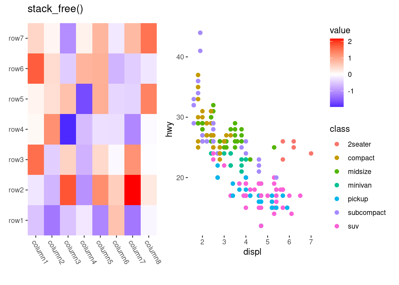
7.6 quad_active()
When you want to resume adding layers (using the "+" operator) to the main heatmap body—after previously adding to an annotation—you need to remove the active context. You can do this using quad_active().
ggheatmap(small_mat) +
    # we set the active context to the top annotation
    anno_top() +
    # we split the observations into 3 groups by hierarchical clustering
    align_dendro(k = 3L) +
    # remove any active annotation
    quad_active() +
    # set fill color scale for the heatmap body
    scale_fill_viridis_c()
#> → heatmap built with `geom_tile()`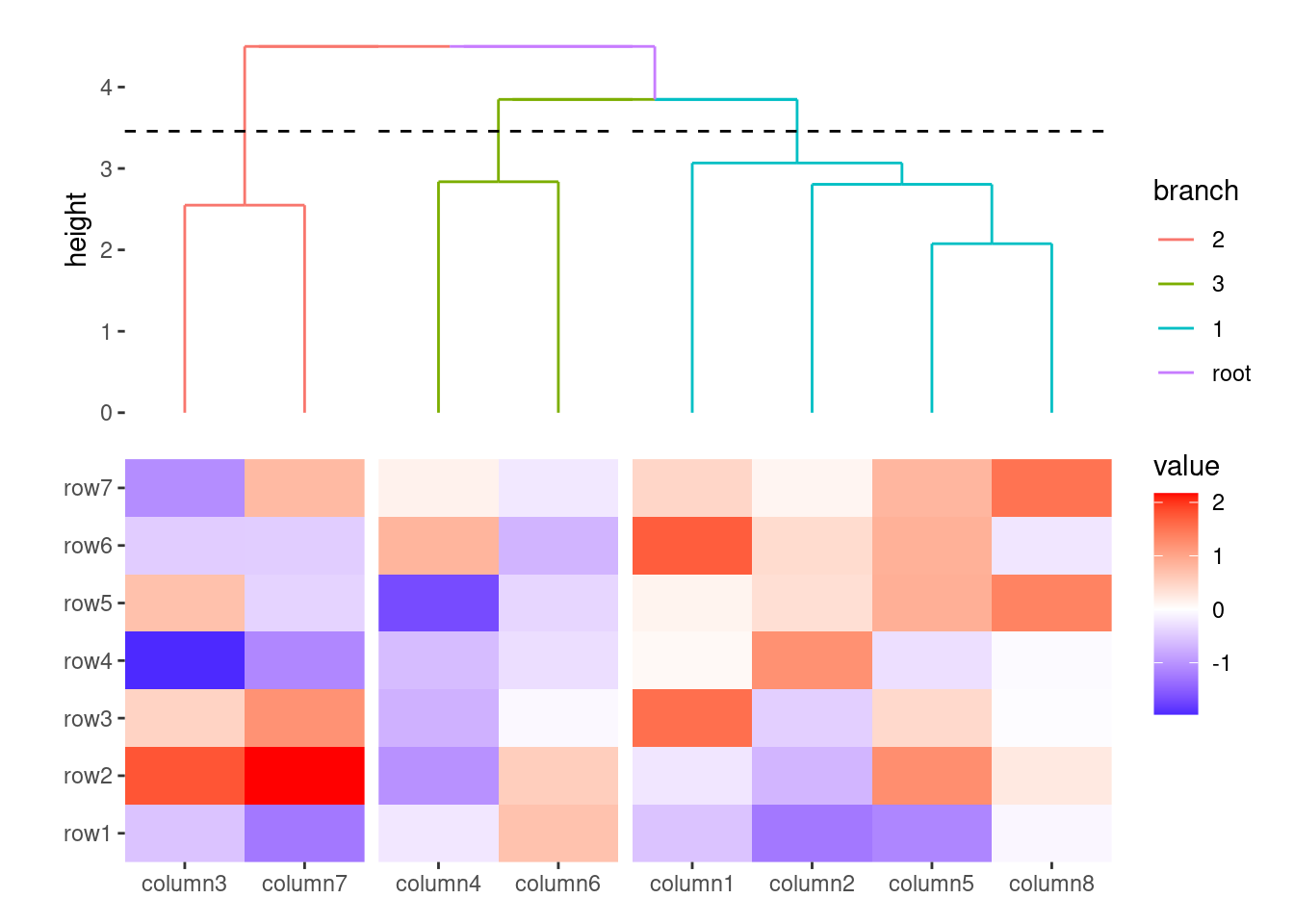
7.7 quad_switch()/hmanno()
We also provide quad_switch()/hmanno() (heatmap annotation) which integrates quad_active() and quad_anno() into one function for ease of use. Feel free to use any of these functions to streamline your annotation process.
ggheatmap(small_mat) +
    # we set the active context to the top annotation
    quad_switch("t") +
    # we split the observations into 3 groups by hierarchical clustering
    align_dendro(k = 3L) +
    # remove any active annotation
    quad_switch() +
    # set fill color scale for the heatmap body
    scale_fill_viridis_c() +
    layout_title("quad_switch()")
#> → heatmap built with `geom_tile()`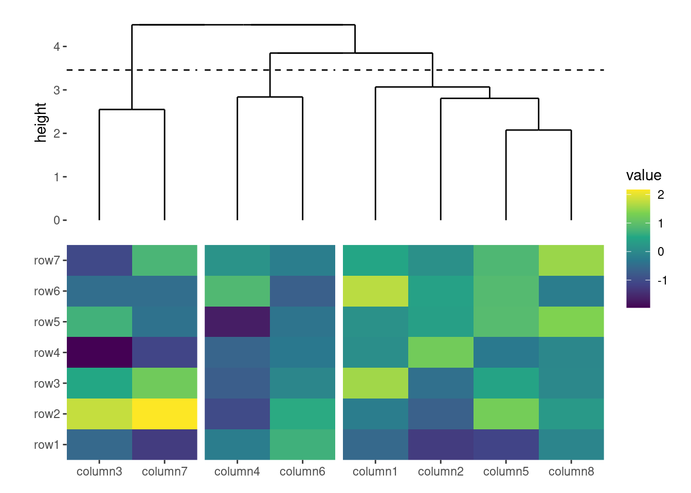
ggheatmap(small_mat) +
    # we set the active context to the top annotation
    hmanno("t") +
    # we split the observations into 3 groups by hierarchical clustering
    align_dendro(k = 3L) +
    # remove any active annotation
    hmanno() +
    # set fill color scale for the heatmap body
    scale_fill_viridis_c()+
    layout_title("hmanno()")
#> → heatmap built with `geom_tile()`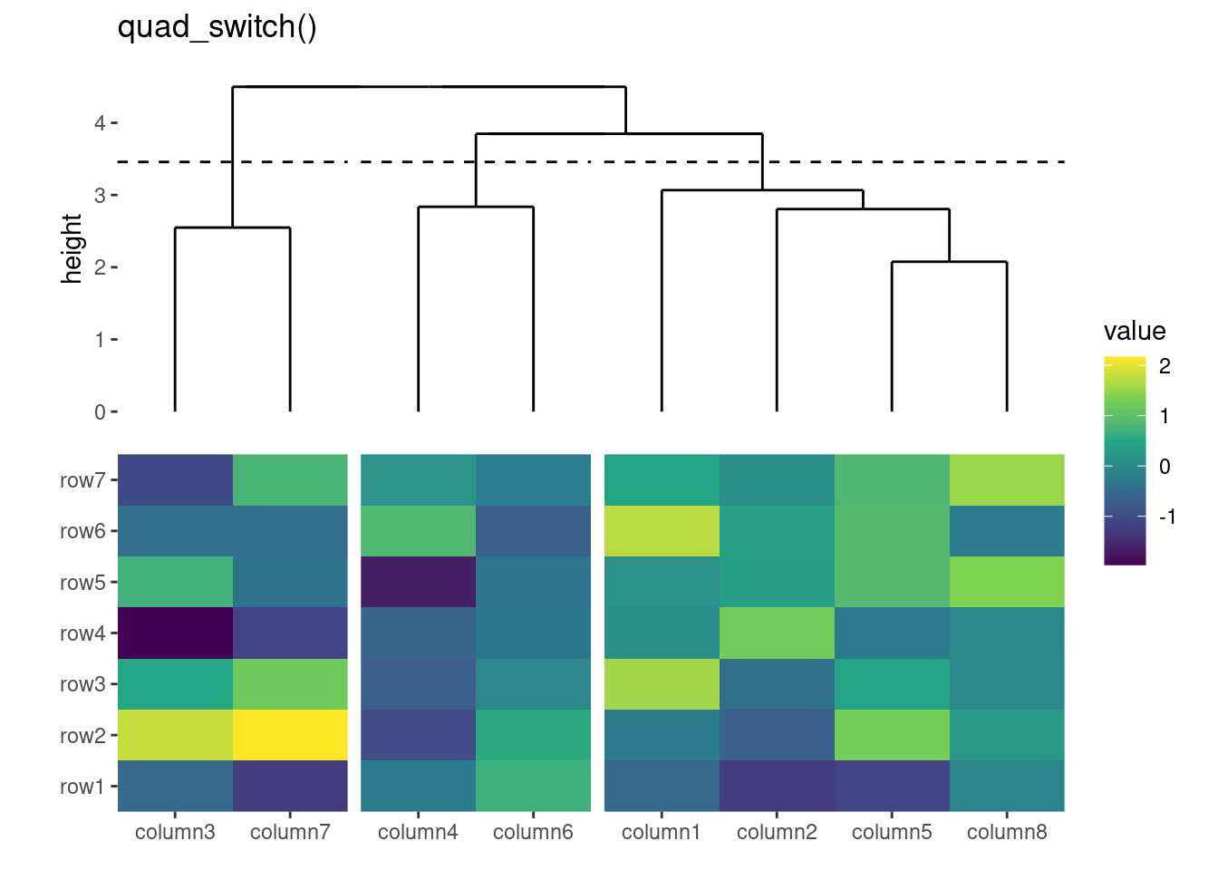
7.8 Plot Size
7.8.1 Heatmap Body Size
You can specify the relative sizes of the heatmap body using the width and height arguments in the ggheatmap() function.
ggheatmap(small_mat, height = 2) +
    anno_top() +
    align_dendro()
#> → heatmap built with `geom_tile()`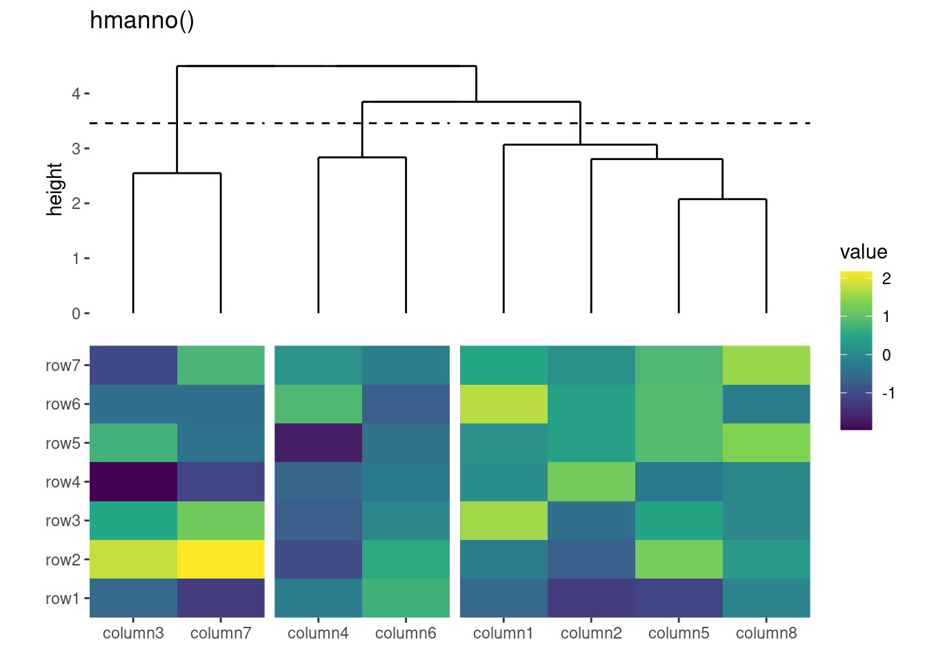
Alternatively, the quad_active() function allows you to control the heatmap body sizes.
ggheatmap(small_mat) +
    quad_active(height = 2) +
    anno_top() +
    align_dendro()
#> → heatmap built with `geom_tile()`
7.8.2 Annotation Stack Size
The quad_anno() function allows you to control the total annotation stack size. The size argument controls the relative width (for left and right annotations) or height (for top and bottom annotations) of the whole annotation stack.
By default, the annotation stack has the same relative size as the heatmap body (height/width). However, if your annotations contain multiple plots, you may need to increase this value to prevent overcrowding:
ggheatmap(small_mat) +
    anno_top(size = 1) +
    align_dendro()
#> → heatmap built with `geom_tile()`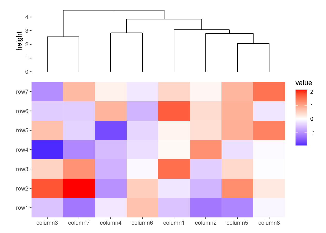
You can also specify it as an absolute size using unit():
ggheatmap(small_mat) +
    anno_top(size = unit(30, "mm")) +
    align_dendro()
#> → heatmap built with `geom_tile()`
Note that the size of an individual plot (Section 6.3) does not affect the total annotation stack size. You must adjust the annotation size using the method described above.
ggheatmap(small_mat) +
    anno_top() +
    align_dendro(size = unit(30, "mm")) +
    layout_title("plot size")
#> → heatmap built with `geom_tile()`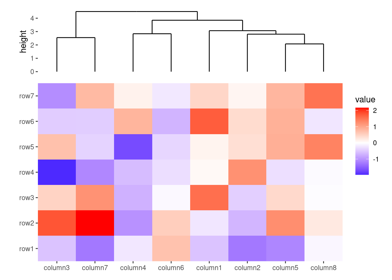
ggheatmap(small_mat) +
    anno_top(size = unit(30, "mm")) +
    align_dendro() +
    layout_title("annotation size")
#> → heatmap built with `geom_tile()`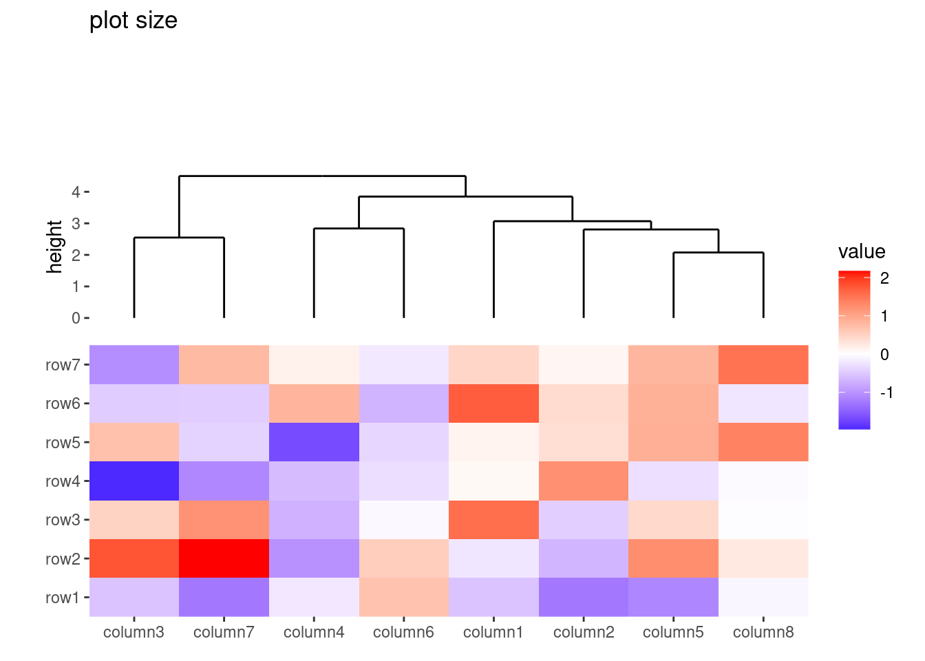
In this chapter, we explored the fundamentals of heatmap layout. These features provide a solid foundation for organizing and visualizing matrix-based data in a structured and interpretable way. As your visualization tasks become more complex—such as requiring precise control over observation ordering or grouping—the need for flexible layout customization becomes increasingly important.
In the next chapter, we’ll introduce layout customization tools that give you full control over the structure and arrangement of your heatmap and annotation components.
