ComplexHeatmap: single-heatmap • ggalign

In this thread, we’ll use ggalign to draw all the heatmap in https://jokergoo.github.io/ComplexHeatmap-reference/book/a-single-heatmap.html

library(ggalign)
#> Loading required package: ggplot2

set.seed(123)
nr1 <- 4
nr2 <- 8
nr3 <- 6
nr <- nr1 + nr2 + nr3
nc1 <- 6
nc2 <- 8
nc3 <- 10
nc <- nc1 + nc2 + nc3
mat <- cbind(
    rbind(
        matrix(rnorm(nr1 * nc1, mean = 1, sd = 0.5), nrow = nr1),
        matrix(rnorm(nr2 * nc1, mean = 0, sd = 0.5), nrow = nr2),
        matrix(rnorm(nr3 * nc1, mean = 0, sd = 0.5), nrow = nr3)
    ),
    rbind(
        matrix(rnorm(nr1 * nc2, mean = 0, sd = 0.5), nrow = nr1),
        matrix(rnorm(nr2 * nc2, mean = 1, sd = 0.5), nrow = nr2),
        matrix(rnorm(nr3 * nc2, mean = 0, sd = 0.5), nrow = nr3)
    ),
    rbind(
        matrix(rnorm(nr1 * nc3, mean = 0.5, sd = 0.5), nrow = nr1),
        matrix(rnorm(nr2 * nc3, mean = 0.5, sd = 0.5), nrow = nr2),
        matrix(rnorm(nr3 * nc3, mean = 1, sd = 0.5), nrow = nr3)
    )
)
mat <- mat[sample(nr, nr), sample(nc, nc)]
rownames(mat) <- paste0("row", seq_len(nr))
colnames(mat) <- paste0("column", seq_len(nc))

Colors

It is important to note that the ComplexHeatmap package reorders the dendrogram by default, while align_dendro() in ggalign does not modify the tree layout.

Another key difference is in how the two packages treat the starting point. ggalign considers the left-bottom as the starting point, whereas ComplexHeatmap starts from the left-top. When reordering the dendrogram, ComplexHeatmap does so in decreasing order, while ggalign uses an ascending order.

To modify colors in the heatmap, you can use the scale_fill_*() function from ggplot2, which provides a flexible way and enriched pallete to adjust color schemes.

# ComplexHeatmap::Heatmap(mat)
dim(mat)
#> [1] 18 24
ggheatmap(mat) +
    theme(axis.text.x = element_text(angle = -60, hjust = 0)) +
    anno_right(size = unit(15, "mm")) +
    align_dendro(reorder_dendrogram = TRUE) +
    anno_top(size = unit(15, "mm")) +
    align_dendro(reorder_dendrogram = TRUE) +
    quad_active() &
    theme(plot.margin = margin())
#> → heatmap built with `geom_tile()`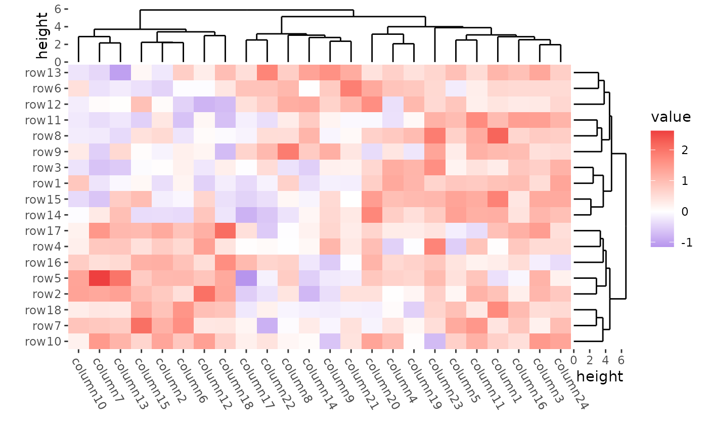

ggheatmap(mat) +
    scale_fill_gradient2(low = "green", high = "red") +
    theme(axis.text.x = element_text(angle = -60, hjust = 0)) +
    anno_right(size = unit(15, "mm")) +
    align_dendro(reorder_dendrogram = TRUE) +
    anno_top(size = unit(15, "mm")) +
    align_dendro() +
    quad_active() &
    theme(plot.margin = margin())
#> → heatmap built with `geom_tile()`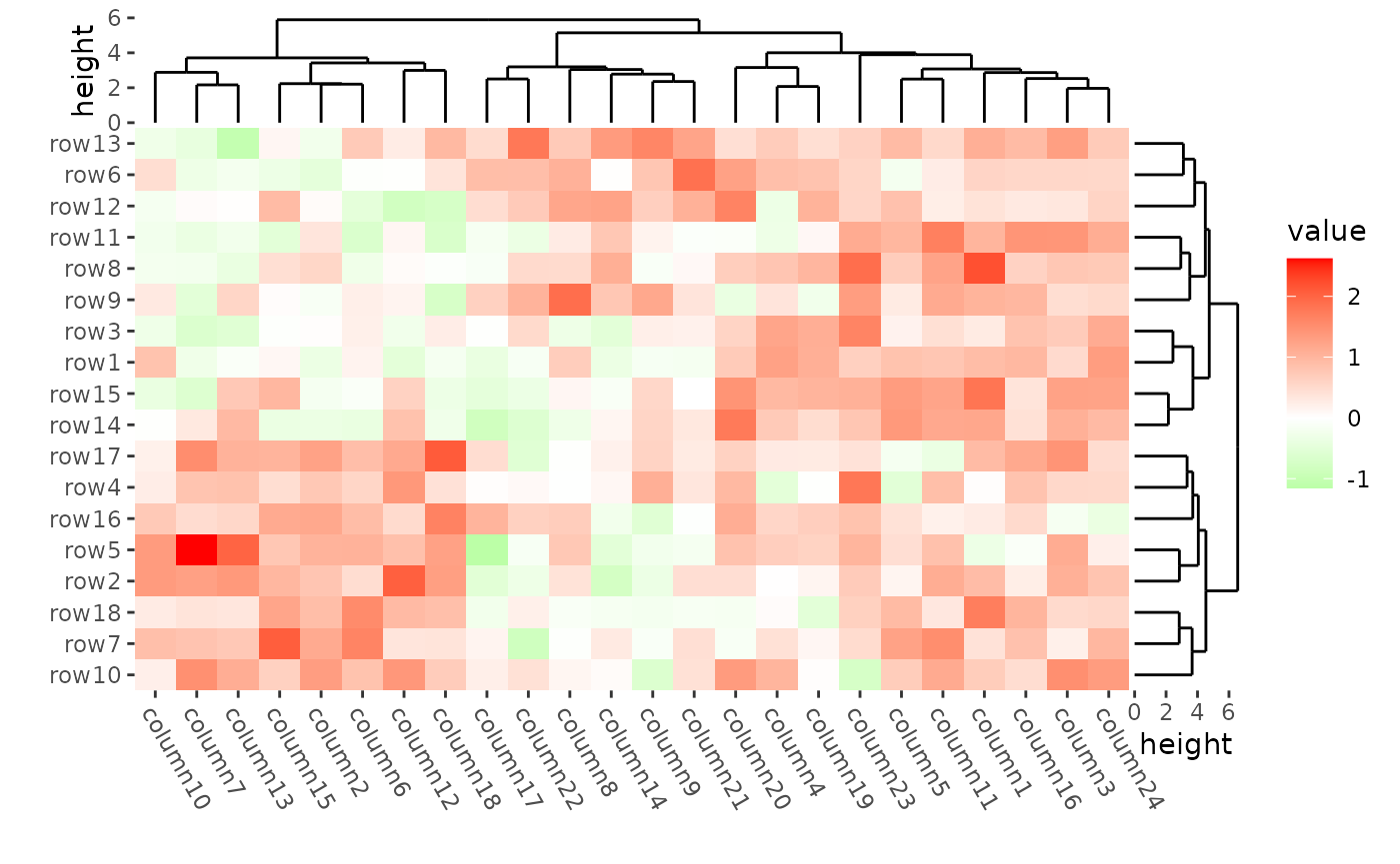

oob argument in the scale_fill_* function can be used to deal with the outliers.

mat2 <- mat
mat2[1, 1] <- 100000
ggheatmap(mat2) +
    scale_fill_gradient2(
        low = "green", high = "red",
        limits = c(-2, 2),
        oob = scales::squish
    ) +
    theme(axis.text.x = element_text(angle = -60, hjust = 0)) +
    anno_right(size = unit(15, "mm")) +
    align_dendro(reorder_dendrogram = TRUE) +
    theme(axis.text.x = element_text(angle = -60, hjust = 0)) +
    anno_top(size = unit(15, "mm")) +
    align_dendro(reorder_dendrogram = TRUE) +
    quad_active() &
    theme(plot.margin = margin())
#> → heatmap built with `geom_tile()`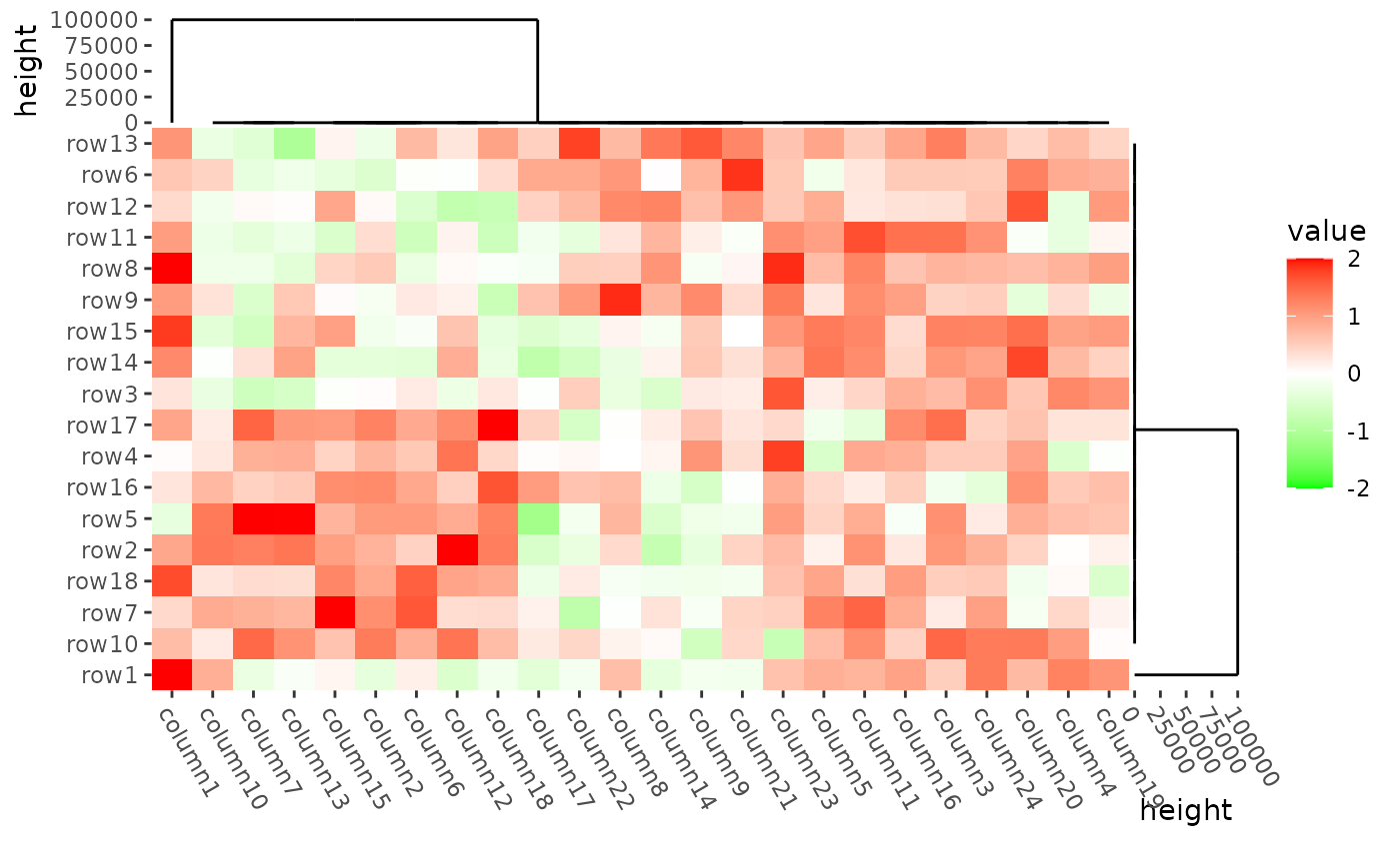

We can use align_plots() to arrange them.

h1 <- ggheatmap(mat) +
    scale_fill_gradient2(name = "mat", low = "green", high = "red") +
    theme(axis.text.x = element_text(angle = -60, hjust = 0)) +
    anno_right(size = unit(15, "mm")) +
    align_dendro(reorder_dendrogram = TRUE) +
    theme(axis.text.x = element_text(angle = -60, hjust = 0)) +
    anno_top(size = unit(15, "mm")) +
    align_dendro(reorder_dendrogram = TRUE) +
    quad_active() &
    theme(plot.margin = margin())

h2 <- ggheatmap(mat / 4) +
    scale_fill_gradient2(
        name = "mat/4", limits = c(-2, 2L),
        oob = scales::squish,
        low = "green", high = "red"
    ) +
    theme(axis.text.x = element_text(angle = -60, hjust = 0)) +
    anno_right(size = unit(15, "mm")) +
    align_dendro(reorder_dendrogram = TRUE) +
    theme(axis.text.x = element_text(angle = -60, hjust = 0)) +
    anno_top(size = unit(15, "mm")) +
    align_dendro(reorder_dendrogram = TRUE) +
    quad_active() &
    theme(plot.margin = margin())

h3 <- ggheatmap(abs(mat)) +
    scale_fill_gradient2(name = "abs(mat)", low = "green", high = "red") +
    theme(axis.text.x = element_text(angle = -60, hjust = 0)) +
    anno_right(size = unit(15, "mm")) +
    align_dendro(reorder_dendrogram = TRUE) +
    theme(axis.text.x = element_text(angle = -60, hjust = 0)) +
    anno_top(size = unit(15, "mm")) +
    align_dendro(reorder_dendrogram = TRUE) +
    quad_active() &
    theme(plot.margin = margin())
align_plots(h1, h2, h3, ncol = 2L)
#> → heatmap built with `geom_tile()`
#> → heatmap built with `geom_tile()`
#> → heatmap built with `geom_tile()`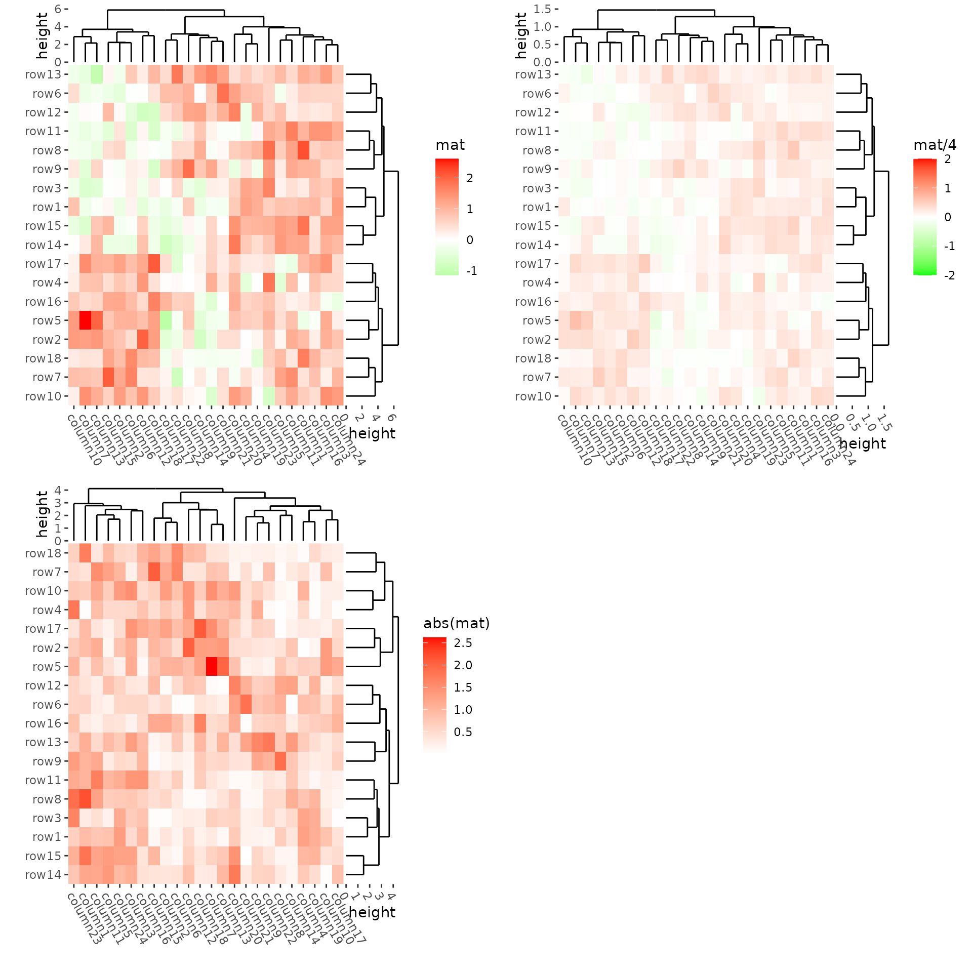

ggheatmap(mat) +
    scale_fill_gradientn(colors = rev(rainbow(10))) +
    theme(axis.text.x = element_text(angle = -60, hjust = 0)) +
    anno_right(size = unit(15, "mm")) +
    align_dendro(reorder_dendrogram = TRUE) +
    anno_top(size = unit(15, "mm")) +
    align_dendro(reorder_dendrogram = TRUE) +
    quad_active() &
    theme(plot.margin = margin())
#> → heatmap built with `geom_tile()`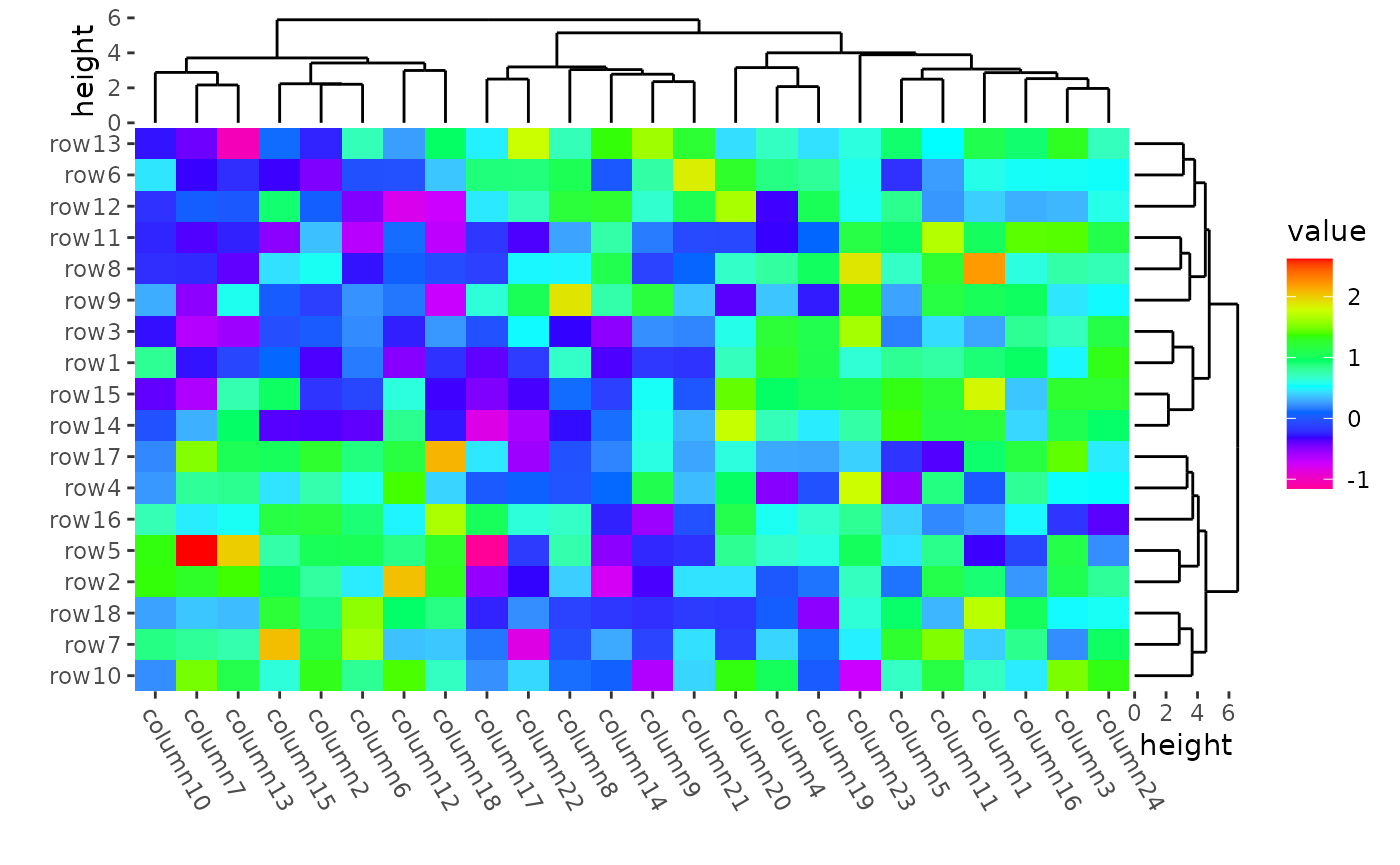

For character matrix, you can use ggplot2 discrete filling scales.

discrete_mat <- matrix(sample(1:4, 100, replace = TRUE), 10, 10)
colors <- structure(1:4, names = c("1", "2", "3", "4")) # black, red, green, blue
ggheatmap(discrete_mat, aes(fill = factor(value))) +
    scale_fill_manual(values = colors) +
    anno_right(size = unit(15, "mm")) +
    align_dendro(reorder_dendrogram = TRUE) +
    anno_top(size = unit(15, "mm")) +
    align_dendro(reorder_dendrogram = TRUE) +
    quad_active() &
    theme(plot.margin = margin())
#> → heatmap built with `geom_tile()`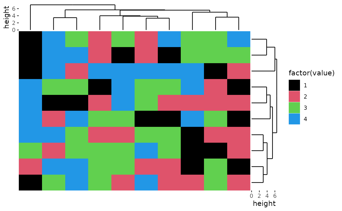

discrete_mat <- matrix(sample(letters[1:4], 100, replace = TRUE), 10, 10)
colors <- structure(1:4, names = letters[1:4])
ggheatmap(discrete_mat) +
    scale_fill_manual(values = colors)
#> → heatmap built with `geom_tile()`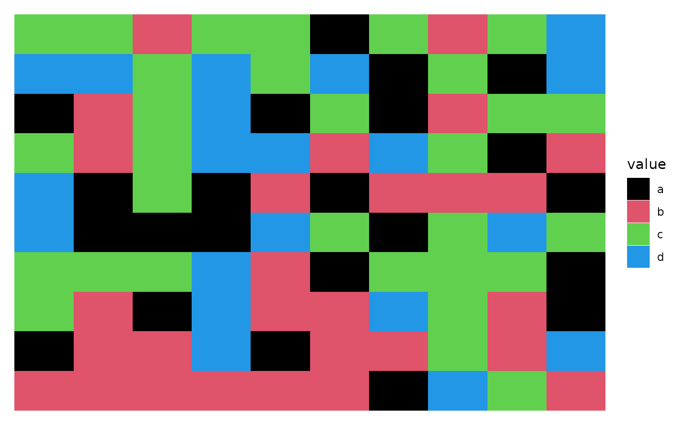

mat_with_na <- mat
na_index <- sample(c(TRUE, FALSE),
    nrow(mat) * ncol(mat),
    replace = TRUE, prob = c(1, 9)
)
mat_with_na[na_index] <- NA
ggheatmap(mat_with_na) +
    scale_fill_gradient2(low = "blue", high = "red", na.value = "black") +
    theme(axis.text.x = element_text(angle = -60, hjust = 0)) +
    anno_right(size = unit(15, "mm")) +
    align_dendro(reorder_dendrogram = TRUE) +
    anno_top(size = unit(15, "mm")) +
    align_dendro(reorder_dendrogram = TRUE) +
    quad_active() &
    theme(plot.margin = margin())
#> → heatmap built with `geom_tile()`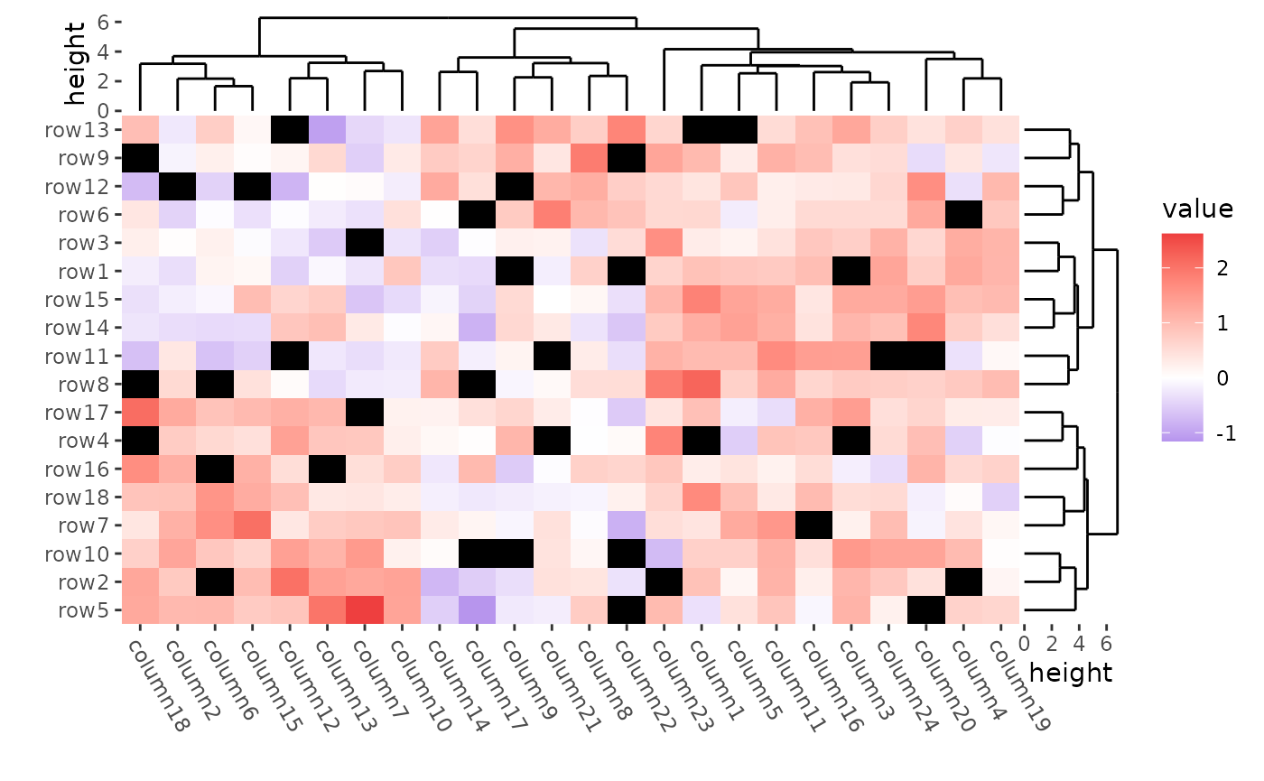

We won’t compare the LAB and RGB space. If you want to convert color between different color space, try to use farver pacakge.

In ggplot2, you can use panel.border argument in theme() function to control the Heatmap body border.

ggheatmap(mat) +
    theme(
        axis.text.x = element_text(angle = -60, hjust = 0),
        panel.border = element_rect(linetype = "dashed", fill = NA)
    ) +
    anno_right(size = unit(15, "mm")) +
    align_dendro(reorder_dendrogram = TRUE) +
    anno_top(size = unit(15, "mm")) +
    align_dendro(reorder_dendrogram = TRUE) +
    theme(plot.margin = margin())
#> → heatmap built with `geom_tile()`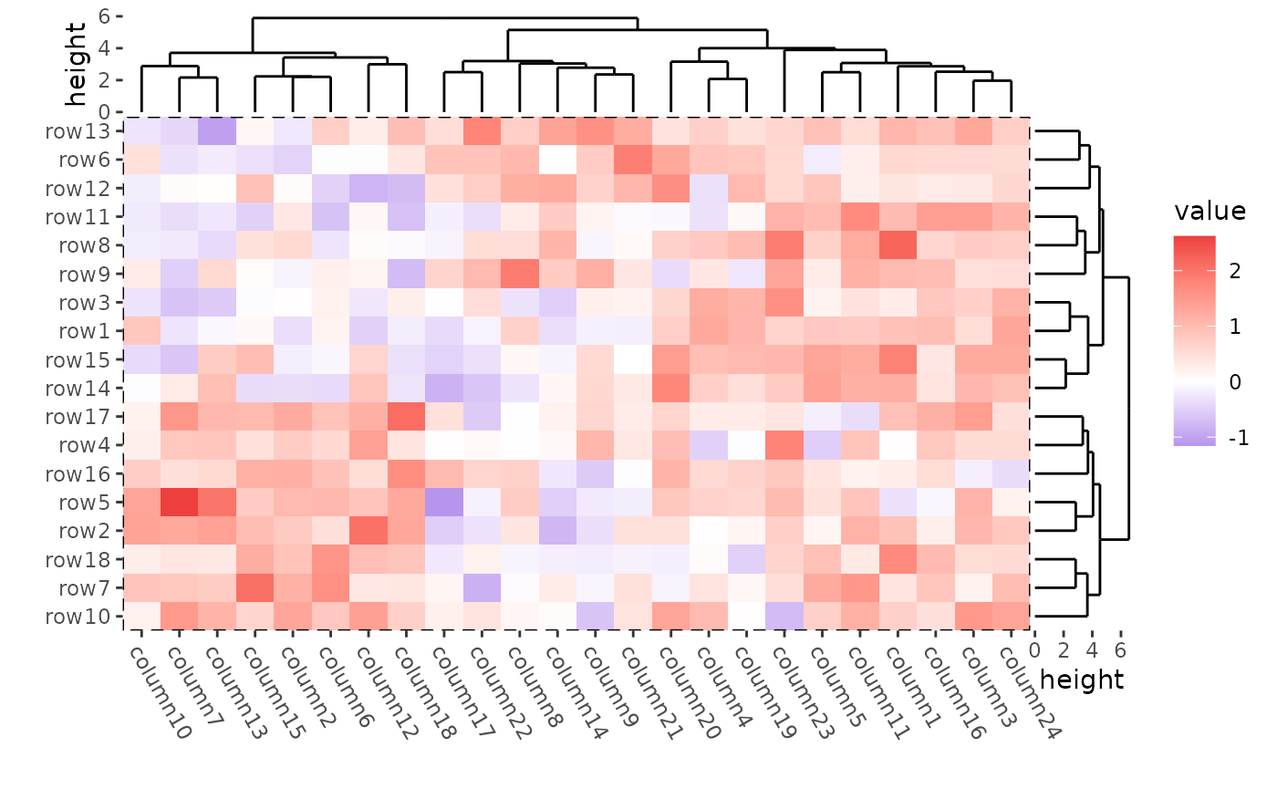

You can use the filling argument to turn off the heatmap cell filling, allowing you to customize the heatmap body geoms. Use the color aesthetic to specify the cell border color and the linewidth aesthetic to set the border width.

ggheatmap(mat, filling = NULL) +
    geom_tile(aes(fill = value), color = "white") +
    theme(axis.text.x = element_text(angle = -60, hjust = 0)) +
    anno_right(size = unit(15, "mm")) +
    align_dendro(reorder_dendrogram = TRUE) +
    anno_top(size = unit(15, "mm")) +
    align_dendro(reorder_dendrogram = TRUE) &
    theme(plot.margin = margin())

To draw a blank heatmap body:

ggheatmap(mat, filling = NULL) +
    theme(axis.text.x = element_text(angle = -60, hjust = 0)) +
    anno_right(size = unit(15, "mm")) +
    align_dendro(reorder_dendrogram = TRUE) +
    anno_top(size = unit(15, "mm")) +
    align_dendro(reorder_dendrogram = TRUE) &
    theme(plot.margin = margin())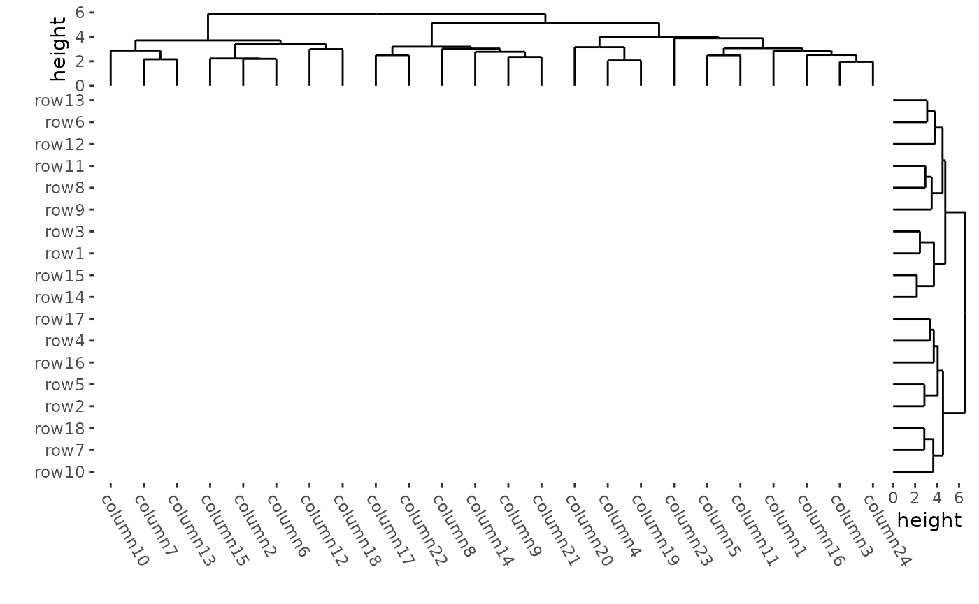

Titles

We can use patch_titles() to add titles around each border of the plot. You can use theme() to control the text appearance.

ggheatmap(mat) +
    theme(axis.text.x = element_text(angle = -60, hjust = 0)) +
    anno_right(size = unit(20, "mm")) +
    align_dendro(reorder_dendrogram = TRUE) +
    patch_titles(right = "I am a row title") +
    theme(plot.patch_title.right = element_text(face = "bold", size = 16)) +
    anno_top(size = unit(15, "mm")) +
    align_dendro(reorder_dendrogram = TRUE) +
    patch_titles(top = "I am a column title") +
    theme(plot.patch_title.top = element_text(face = "bold", size = 16)) &
    theme(plot.margin = margin())
#> → heatmap built with `geom_tile()`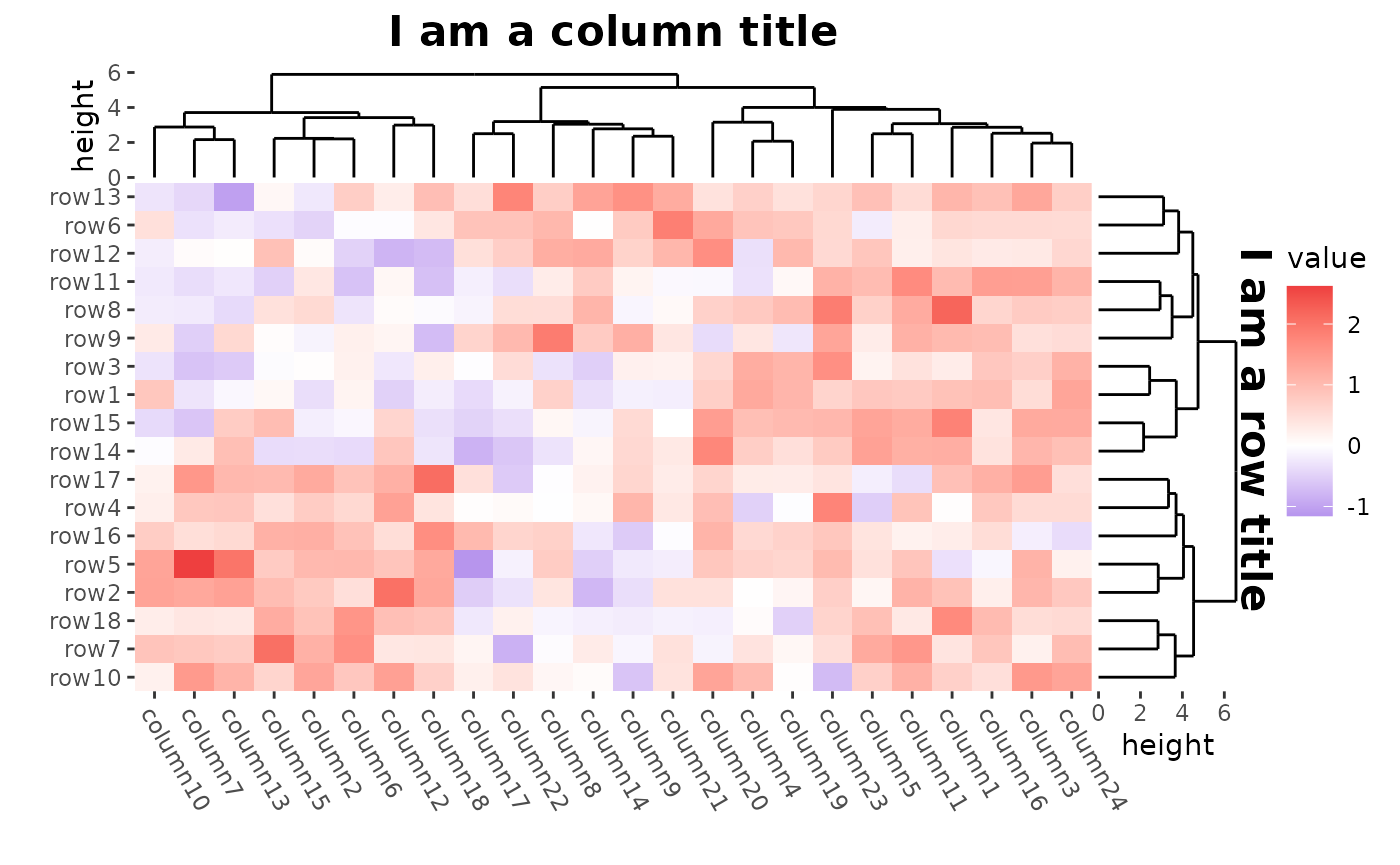

Clustering

Distance methods

# ComplexHeatmap::Heatmap(mat,
#   name = "mat", clustering_distance_rows = "pearson",
#   column_title = "pre-defined distance method (1 - pearson)"
# )
ggheatmap(mat) +
    theme(axis.text.x = element_text(angle = -60, hjust = 0)) +
    anno_right(size = unit(20, "mm")) +
    align_dendro(distance = "pearson", reorder_dendrogram = TRUE) +
    anno_top(size = unit(15, "mm")) +
    align_dendro(reorder_dendrogram = TRUE) +
    patch_titles(top = "pre-defined distance method (1 - pearson)") +
    theme(plot.patch_title.top = element_text(face = "bold", size = 16)) &
    theme(plot.margin = margin())
#> → heatmap built with `geom_tile()`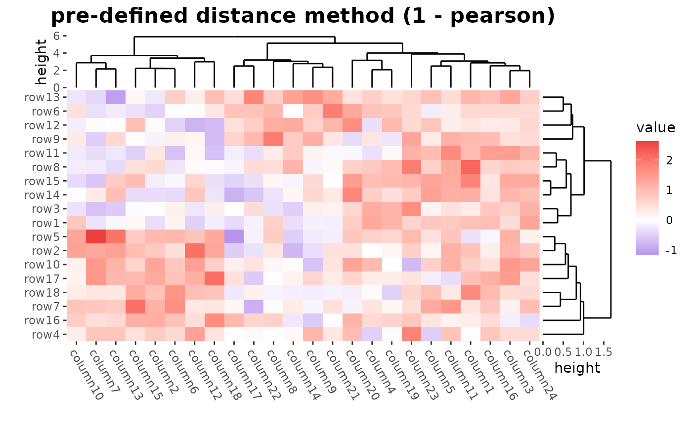

# ComplexHeatmap::Heatmap(mat,
#     name = "mat", clustering_distance_rows = function(m) dist(m),
#     column_title = "a function that calculates distance matrix"
# )
ggheatmap(mat) +
    theme(axis.text.x = element_text(angle = -60, hjust = 0)) +
    anno_right(size = unit(20, "mm")) +
    align_dendro(distance = dist, reorder_dendrogram = TRUE) +
    anno_top(size = unit(15, "mm")) +
    align_dendro(reorder_dendrogram = TRUE) +
    patch_titles(top = "a function that calculates distance matrix") +
    theme(plot.patch_title.top = element_text(face = "bold", size = 16)) &
    theme(plot.margin = margin())
#> → heatmap built with `geom_tile()`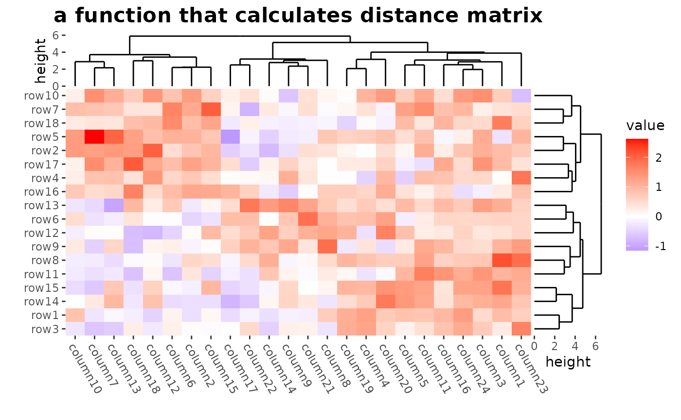

Clustering methods

Method to perform hierarchical clustering can be specified by method argument, Possible methods are those supported in hclust() function.

# ComplexHeatmap::Heatmap(mat,
#     name = "mat",
#     clustering_method_rows = "single"
# )
ggheatmap(mat) +
    theme(axis.text.x = element_text(angle = -60, hjust = 0)) +
    anno_right(size = unit(20, "mm")) +
    align_dendro(method = "single", reorder_dendrogram = TRUE) +
    anno_top(size = unit(15, "mm")) +
    align_dendro(reorder_dendrogram = TRUE) &
    theme(plot.margin = margin())
#> → heatmap built with `geom_tile()`

Use distance = NULL if you don’t want to calculate the distance.

ggheatmap(mat) +
    theme(axis.text.x = element_text(angle = -60, hjust = 0)) +
    anno_right(size = unit(20, "mm")) +
    align_dendro(
        distance = NULL, method = cluster::diana,
        reorder_dendrogram = TRUE
    ) +
    anno_top(size = unit(15, "mm")) +
    align_dendro(
        distance = NULL, method = cluster::agnes,
        reorder_dendrogram = TRUE
    ) &
    theme(plot.margin = margin())
#> → heatmap built with `geom_tile()`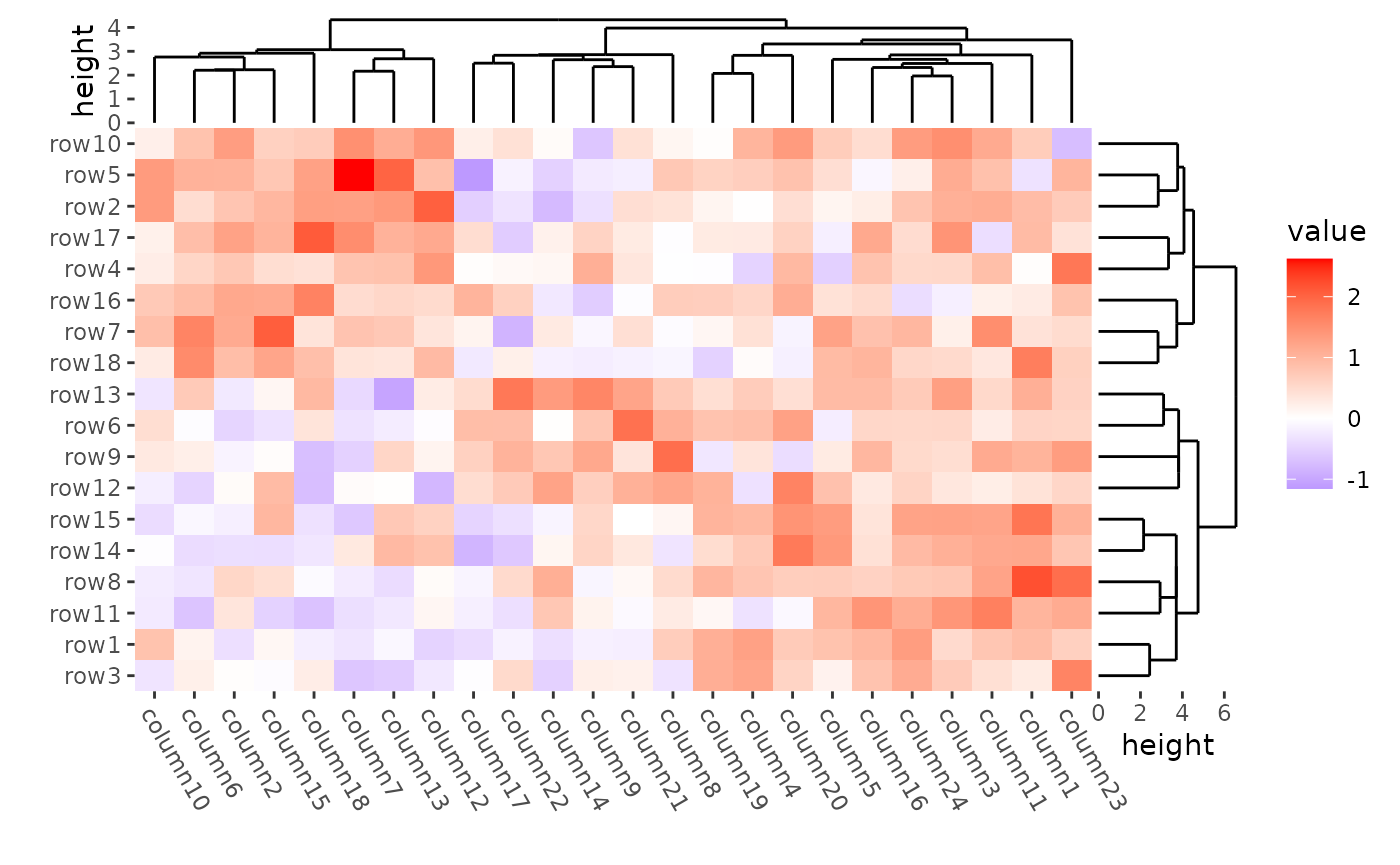

Render dendrograms

It’s easy for ggalign to color the branches by setting the color mapping, since ggalign will add the cutree() results into the underlying data.

ggheatmap(mat) +
    theme(axis.text.x = element_text(angle = -60, hjust = 0)) +
    anno_right(size = unit(20, "mm")) +
    align_dendro(aes(color = branch), k = 2L, reorder_dendrogram = TRUE) +
    anno_top(size = unit(15, "mm")) +
    align_dendro(reorder_dendrogram = TRUE) &
    theme(plot.margin = margin())
#> → heatmap built with `geom_tile()`

Set row and column orders

We can use align_order() to set the order.

# ComplexHeatmap::Heatmap(mat,
#     name = "mat",
#     row_order = order(as.numeric(gsub("row", "", rownames(mat)))),
#     column_order = order(as.numeric(gsub("column", "", colnames(mat)))),
#     column_title = "reorder matrix"
# )
ggheatmap(mat) +
    theme(axis.text.x = element_text(angle = -60, hjust = 0)) +
    anno_right(size = unit(20, "mm")) +
    align_order(as.numeric(gsub("row", "", rownames(mat)))) +
    anno_top(size = unit(15, "mm")) +
    align_order(as.numeric(gsub("column", "", colnames(mat)))) &
    theme(plot.margin = margin())
#> → heatmap built with `geom_tile()`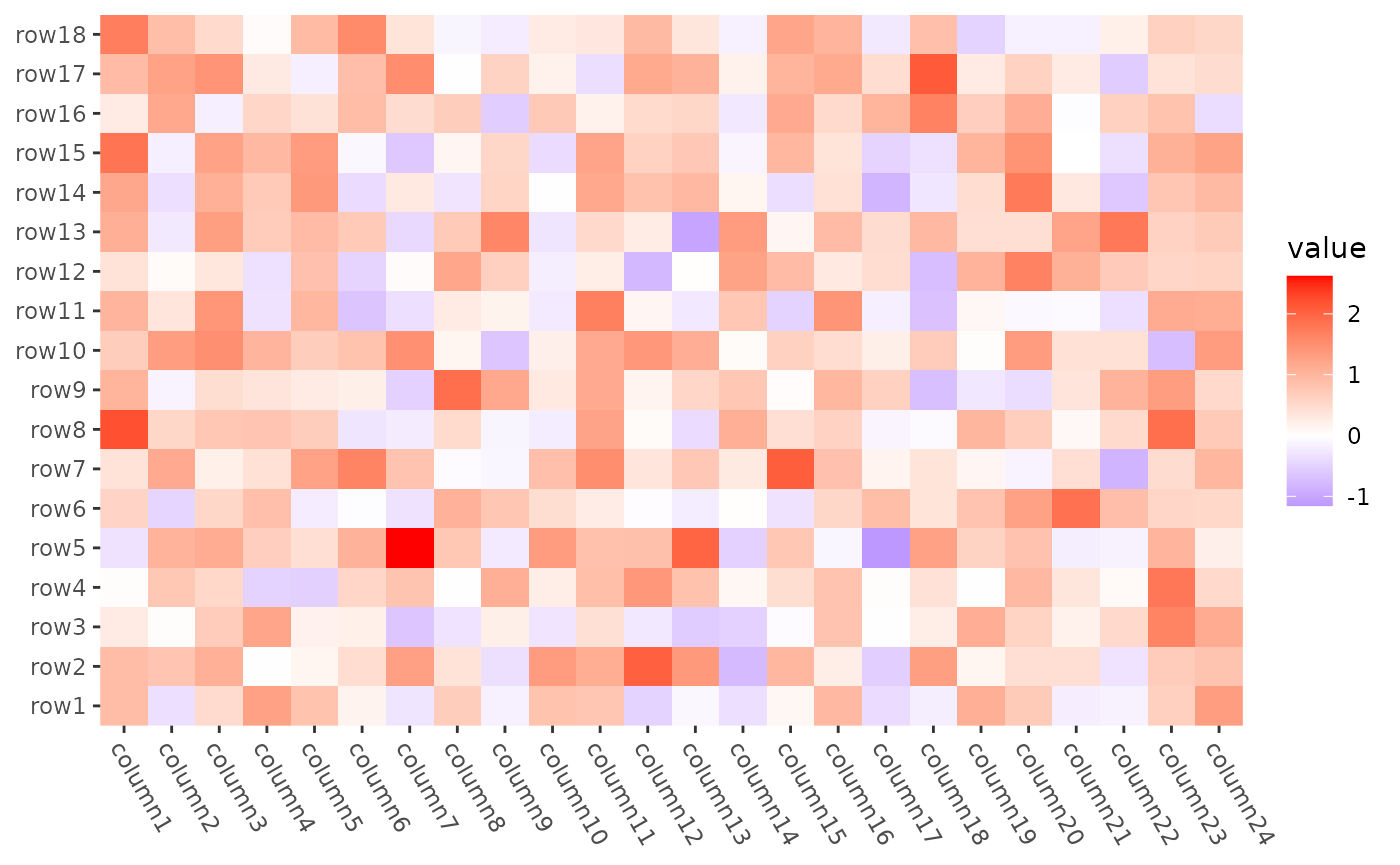

Seriation

align_reorder() can directly take the seriate() function as the input and extract the ordering information.

mat2 <- max(mat) - mat
ggheatmap(mat2) +
    scale_fill_gradient2(low = "blue", high = "red", midpoint = 2L) +
    theme(axis.text.x = element_text(angle = -60, hjust = 0)) +
    anno_right(size = unit(20, "mm")) +
    align_reorder(seriation::seriate, method = "BEA_TSP") +
    anno_top(size = unit(15, "mm")) +
    align_reorder(seriation::seriate, method = "BEA_TSP") &
    theme(plot.margin = margin())
#> → heatmap built with `geom_tile()`

The above code will execute seriate() twice—once for each dimension. However, since a single run of seriate() can provide the ordering for both dimensions, we can manually extract the ordering indices to avoid redundancy.

o <- seriation::seriate(mat2, method = "BEA_TSP")
ggheatmap(mat2) +
    scale_fill_gradient2(low = "blue", high = "red", midpoint = 2L) +
    theme(axis.text.x = element_text(angle = -60, hjust = 0)) +
    anno_right(size = unit(20, "mm")) +
    align_order(seriation::get_order(o, 1L)) +
    anno_top(size = unit(15, "mm")) +
    align_order(seriation::get_order(o, 2L)) &
    theme(plot.margin = margin())
#> → heatmap built with `geom_tile()`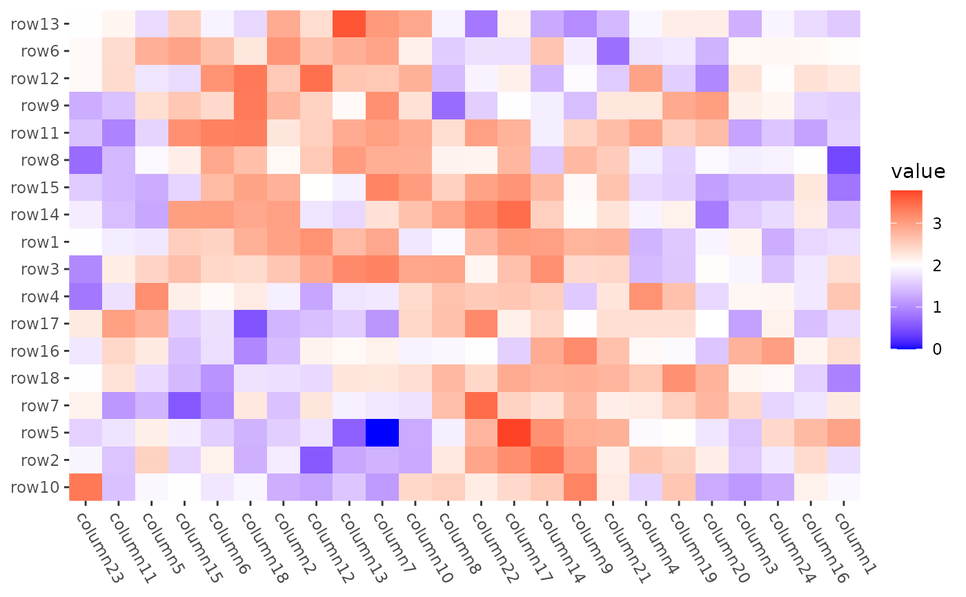

For more use of the seriate() function, please refer to the seriation package.

Dimension labels

ggplot2 use scales and theme to control the axis labels, Please see scales section for more details.

# ComplexHeatmap::Heatmap(mat,
#     name = "mat", row_names_side = "left", row_dend_side = "right",
#     column_names_side = "top", column_dend_side = "bottom"
# )
ggheatmap(mat) +
    scale_x_continuous(position = "top") +
    scale_y_continuous(position = "right") +
    theme(axis.text.x = element_text(angle = 60, hjust = 0)) +
    anno_left(size = unit(15, "mm")) +
    align_dendro(reorder_dendrogram = TRUE) +
    scale_x_continuous(position = "top") +
    anno_bottom(size = unit(15, "mm")) +
    align_dendro(reorder_dendrogram = TRUE) +
    scale_y_continuous(position = "right") +
    quad_active() &
    theme(plot.margin = margin())
#> → heatmap built with `geom_tile()`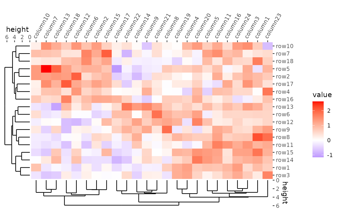

ggheatmap(mat) +
    scale_y_continuous(breaks = NULL) +
    theme(axis.text.x = element_text(angle = -60, hjust = 0)) +
    anno_right(size = unit(15, "mm")) +
    align_dendro(reorder_dendrogram = TRUE) +
    anno_top(size = unit(15, "mm")) +
    align_dendro(reorder_dendrogram = TRUE) +
    quad_active() &
    theme(plot.margin = margin())
#> → heatmap built with `geom_tile()`

ggheatmap(mat) +
    theme(
        axis.text.x = element_text(angle = -60, hjust = 0),
        axis.text.y = element_text(face = "bold", size = 16)
    ) +
    anno_right(size = unit(15, "mm")) +
    align_dendro(reorder_dendrogram = TRUE) +
    anno_top(size = unit(15, "mm")) +
    align_dendro(reorder_dendrogram = TRUE) +
    quad_active() &
    theme(plot.margin = margin())
#> → heatmap built with `geom_tile()`

ggheatmap(mat) +
    theme(
        axis.text.x = element_text(angle = -60, hjust = 0),
        axis.text.y = element_text(
            face = "bold", size = 16,
            colour = c(rep("red", 10), rep("blue", 8))
        )
    ) +
    anno_right(size = unit(15, "mm")) +
    align_dendro(reorder_dendrogram = TRUE) +
    anno_top(size = unit(15, "mm")) +
    align_dendro(reorder_dendrogram = TRUE) +
    quad_active() &
    theme(plot.margin = margin())
#> Warning: Vectorized input to `element_text()` is not officially supported.
#> ℹ Results may be unexpected or may change in future versions of ggplot2.
#> → heatmap built with `geom_tile()`

Heatmap split

Split by k-means clustering

ggheatmap(mat) +
    theme(axis.text.x = element_text(angle = -60, hjust = 0)) +
    anno_right(size = unit(15, "mm")) +
    align_kmeans(2L) +
    align_dendro(reorder_dendrogram = TRUE) +
    anno_top(size = unit(15, "mm")) +
    align_dendro(reorder_dendrogram = TRUE) +
    quad_active() &
    theme(plot.margin = margin())
#> → heatmap built with `geom_tile()`

ggheatmap(mat) +
    theme(axis.text.x = element_text(angle = -60, hjust = 0)) +
    anno_right(size = unit(15, "mm")) +
    align_dendro(reorder_dendrogram = TRUE) +
    anno_top(size = unit(15, "mm")) +
    align_kmeans(3L) +
    align_dendro(reorder_dendrogram = TRUE) +
    quad_active() &
    theme(plot.margin = margin())
#> → heatmap built with `geom_tile()`

ggheatmap(mat) +
    theme(axis.text.x = element_text(angle = -60, hjust = 0)) +
    anno_right(size = unit(15, "mm")) +
    align_kmeans(2L) +
    align_dendro(reorder_dendrogram = TRUE) +
    anno_top(size = unit(15, "mm")) +
    align_kmeans(3L) +
    align_dendro(reorder_dendrogram = TRUE) +
    quad_active() &
    theme(plot.margin = margin())
#> → heatmap built with `geom_tile()`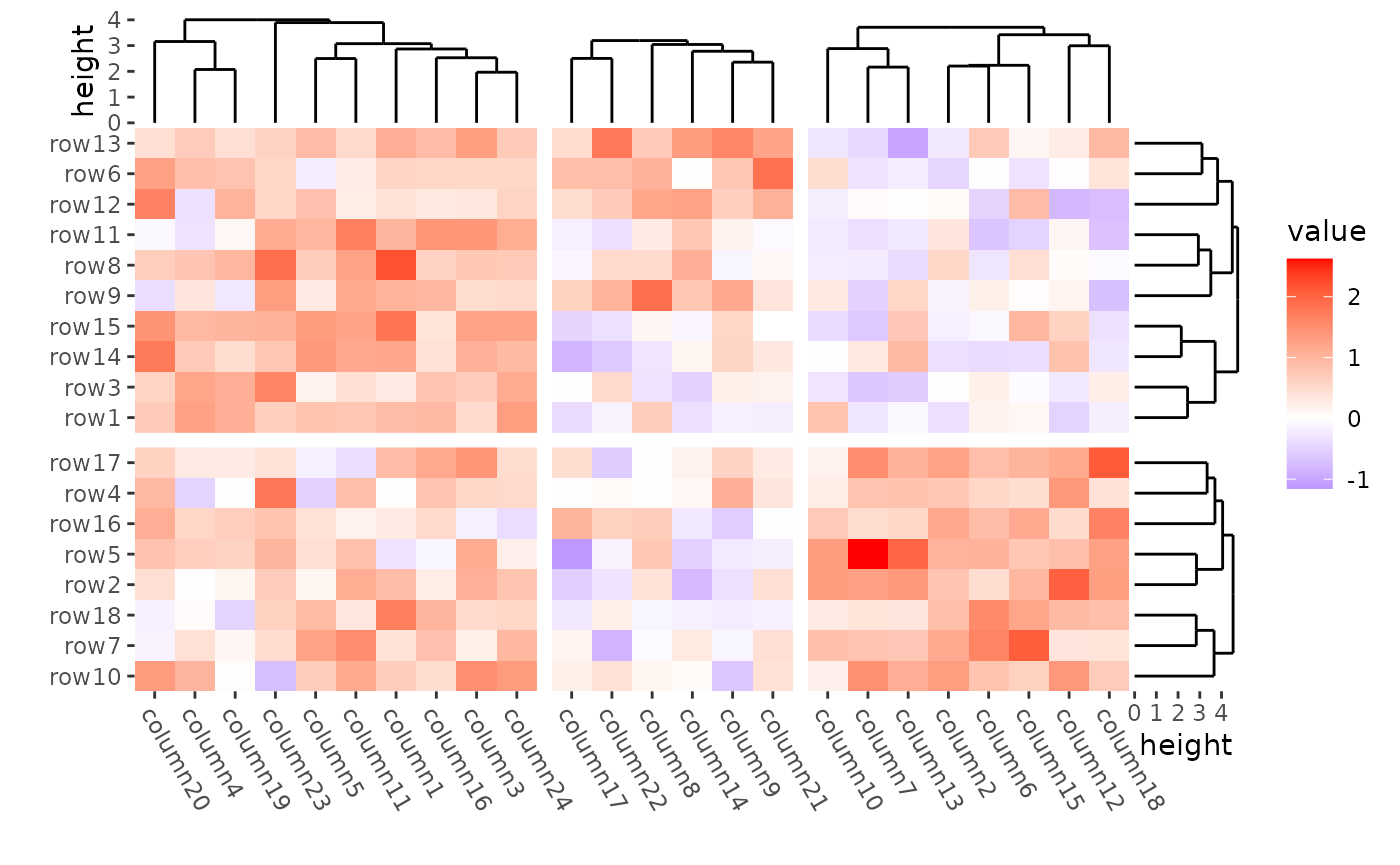

The dendrogram was calculated in each group defined by kmeans.

Split by categorical variables

ggheatmap(mat) +
    theme(axis.text.x = element_text(angle = -60, hjust = 0)) +
    anno_right(size = unit(15, "mm")) +
    align_group(rep(c("A", "B"), 9)) +
    align_dendro(reorder_dendrogram = TRUE) +
    anno_top(size = unit(15, "mm")) +
    align_group(rep(c("C", "D"), 12)) +
    align_dendro(reorder_dendrogram = TRUE) +
    quad_active() &
    theme(plot.margin = margin())
#> → heatmap built with `geom_tile()`

Split by dendrogram

When you splitted by a dendrogram, the cutted height will be indicated with a dashed line.

ggheatmap(mat) +
    theme(axis.text.x = element_text(angle = -60, hjust = 0)) +
    anno_right(size = unit(15, "mm")) +
    align_dendro(k = 3L, reorder_dendrogram = TRUE) +
    anno_top(size = unit(15, "mm")) +
    align_dendro(k = 2L, reorder_dendrogram = TRUE) +
    quad_active() &
    theme(plot.margin = margin())
#> → heatmap built with `geom_tile()`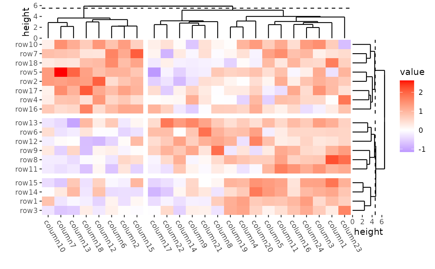

ggheatmap(mat) +
    theme(axis.text.x = element_text(angle = -60, hjust = 0)) +
    anno_right(size = unit(15, "mm")) +
    align_dendro(aes(color = branch), k = 3L, reorder_dendrogram = TRUE) +
    scale_color_brewer(palette = "Dark2") +
    anno_top(size = unit(15, "mm")) +
    align_dendro(k = 2L, reorder_dendrogram = TRUE) +
    quad_active() &
    theme(plot.margin = margin())
#> → heatmap built with `geom_tile()`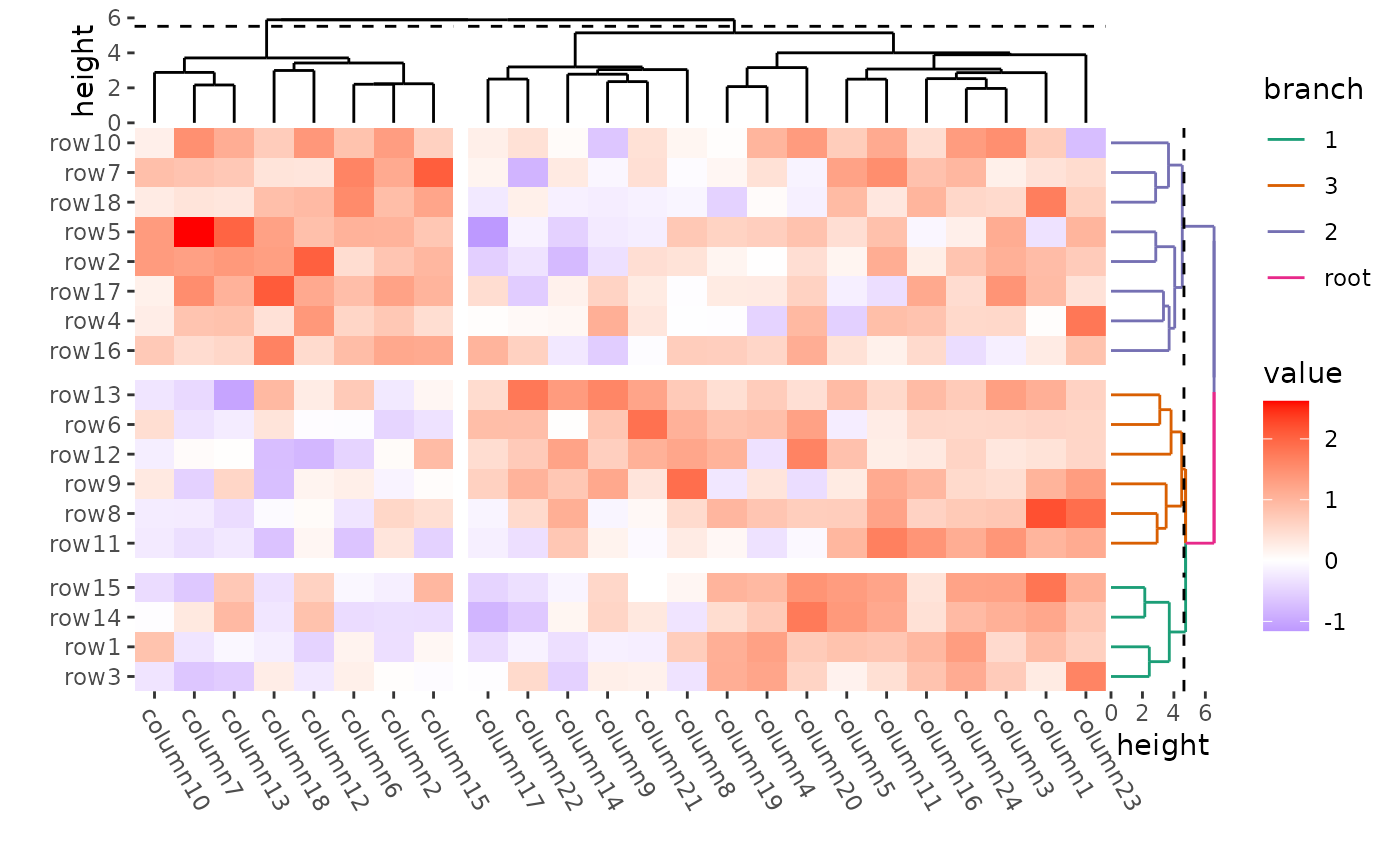

Order of slices (panels)

The order of the panels always follow the factor level. Note: the merging of dendrogram between ComplexHeatmap and ggalign is a little different.

ggheatmap(mat) +
    theme(axis.text.x = element_text(angle = -60, hjust = 0)) +
    anno_right(size = unit(15, "mm")) +
    align_group(rep(LETTERS[1:3], 6)) +
    align_dendro(aes(color = branch),
        reorder_dendrogram = TRUE,
        reorder_group = TRUE,
        merge_dendrogram = TRUE
    ) +
    scale_color_brewer(palette = "Dark2") +
    anno_top(size = unit(15, "mm")) +
    align_group(rep(letters[1:6], 4)) +
    align_dendro(aes(color = branch),
        reorder_dendrogram = TRUE,
        reorder_group = TRUE,
        merge_dendrogram = TRUE
    ) +
    quad_active() -
    with_quad(theme(strip.text = element_text()), "tr") &
    theme(plot.margin = margin())
#> → heatmap built with `geom_tile()`

ggheatmap(mat) +
    theme(axis.text.x = element_text(angle = -60, hjust = 0)) +
    anno_right(size = unit(15, "mm")) +
    align_group(rep(LETTERS[1:3], 6)) +
    align_dendro(aes(color = branch), reorder_dendrogram = TRUE) +
    scale_color_brewer(palette = "Dark2") +
    anno_top(size = unit(15, "mm")) +
    align_group(rep(letters[1:6], 4)) +
    align_dendro(aes(color = branch), reorder_dendrogram = TRUE) +
    quad_active() -
    with_quad(theme(strip.text = element_text()), "tr") &
    theme(plot.margin = margin())
#> → heatmap built with `geom_tile()`

Titles for splitting (facet strip text)

By default, the facet strip text is removed. You can override this behavior with theme(strip.text = element_text()). Since align_group() does not create a new plot, the panel title can only be added to the heatmap plot.

waiting for complete …

Graphic parameters for splitting

ggh4x::facet_grid2(strip = ggh4x::strip_themed(
    background_x = list(
        element_rect(fill = "red"),
        element_rect(fill = "blue"),
        element_rect(fill = "green")
    )
))
#> <ggproto object: Class FacetGrid2, FacetGrid, Facet, gg>
#>     attach_axes: function
#>     compute_layout: function
#>     draw_back: function
#>     draw_front: function
#>     draw_labels: function
#>     draw_panels: function
#>     finish_data: function
#>     finish_panels: function
#>     init_scales: function
#>     map_data: function
#>     params: list
#>     setup_aspect_ratio: function
#>     setup_axes: function
#>     setup_data: function
#>     setup_panel_table: function
#>     setup_params: function
#>     shrink: TRUE
#>     strip: <ggproto object: Class StripElemental, Strip, gg>
#>         assemble_strip: function
#>         build_strip: function
#>         clip: inherit
#>         draw_labels: function
#>         elements: list
#>         finish_strip: function
#>         get_strips: function
#>         given_elements: list
#>         incorporate_grid: function
#>         incorporate_wrap: function
#>         init_strip: function
#>         params: list
#>         setup: function
#>         setup_elements: function
#>         strips: list
#>         super:  <ggproto object: Class StripElemental, Strip, gg>
#>     train_scales: function
#>     vars: function
#>     vars_combine: function
#>     super:  <ggproto object: Class FacetGrid2, FacetGrid, Facet, gg>

Session information

sessionInfo()
#> R version 4.4.2 (2024-10-31)
#> Platform: x86_64-pc-linux-gnu
#> Running under: Ubuntu 22.04.5 LTS
#> 
#> Matrix products: default
#> BLAS:   /usr/lib/x86_64-linux-gnu/openblas-pthread/libblas.so.3 
#> LAPACK: /usr/lib/x86_64-linux-gnu/openblas-pthread/libopenblasp-r0.3.20.so;  LAPACK version 3.10.0
#> 
#> locale:
#>  [1] LC_CTYPE=C.UTF-8       LC_NUMERIC=C           LC_TIME=C.UTF-8       
#>  [4] LC_COLLATE=C.UTF-8     LC_MONETARY=C.UTF-8    LC_MESSAGES=C.UTF-8   
#>  [7] LC_PAPER=C.UTF-8       LC_NAME=C              LC_ADDRESS=C          
#> [10] LC_TELEPHONE=C         LC_MEASUREMENT=C.UTF-8 LC_IDENTIFICATION=C   
#> 
#> time zone: UTC
#> tzcode source: system (glibc)
#> 
#> attached base packages:
#> [1] stats     graphics  grDevices utils     datasets  methods   base     
#> 
#> other attached packages:
#> [1] ggalign_0.0.5 ggplot2_3.5.1
#> 
#> loaded via a namespace (and not attached):
#>  [1] gtable_0.3.6       jsonlite_1.8.9     dplyr_1.1.4        compiler_4.4.2    
#>  [5] tidyselect_1.2.1   cluster_2.1.6      jquerylib_0.1.4    systemfonts_1.1.0 
#>  [9] scales_1.3.0       textshaping_0.4.0  ggh4x_0.2.8        yaml_2.3.10       
#> [13] fastmap_1.2.0      R6_2.5.1           labeling_0.4.3     generics_0.1.3    
#> [17] ca_0.71.1          knitr_1.49         iterators_1.0.14   tibble_3.2.1      
#> [21] desc_1.4.3         munsell_0.5.1      RColorBrewer_1.1-3 bslib_0.8.0       
#> [25] pillar_1.9.0       rlang_1.1.4        utf8_1.2.4         cachem_1.1.0      
#> [29] xfun_0.49          fs_1.6.5           sass_0.4.9         TSP_1.2-4         
#> [33] registry_0.5-1     cli_3.6.3          withr_3.0.2        pkgdown_2.1.1     
#> [37] magrittr_2.0.3     digest_0.6.37      foreach_1.5.2      grid_4.4.2        
#> [41] lifecycle_1.0.4    vctrs_0.6.5        evaluate_1.0.1     glue_1.8.0        
#> [45] farver_2.1.2       codetools_0.2-20   ragg_1.3.3         fansi_1.0.6       
#> [49] colorspace_2.1-1   rmarkdown_2.29     seriation_1.5.6    pkgconfig_2.0.3   
#> [53] tools_4.4.2        htmltools_0.5.8.1